Week 15 — Final review & synthesis

The whole commuter’s-morning thread as one picture

The week question

We have spent fourteen weeks adding machinery one piece at a time, and each piece arrived wired to the same small world: Maya’s commuter morning. This last class is not for new tools. It is for stepping back far enough to see that the tools were never separate — they were a single chain of reasoning that grew one link at a time. So the question this week is the most useful one you can ask before a cumulative final: when a probability problem lands in front of you, how do you know which idea it is asking for, and how do the ideas connect?

The honest answer is that almost every problem in this course is one of a handful of moves — describe the randomness, condition on what you know, update a belief, count or model the variable, summarize it with a mean and spread, fit a named distribution, or take a limit — and the whole term has been those moves applied to one running story. If you can re-walk Maya’s morning end to end and name the move at each step, you can read almost any first-course probability problem. That re-walk is what this page is.

Why this matters

A final exam tempts you to memorize formulas. That is the wrong instinct, and this course was built to push back on it. The reason naming a distribution mattered in Week 9, or stating an assumption out loud mattered in Week 4, is that the hard part of a probability problem is almost never the arithmetic — it is deciding what kind of object you are holding. Is “rain this morning” an event or a random variable? Is the question asking for a marginal probability, a conditional one, or an updated one? Is the wait time discrete or continuous? Get those choices right and the formula is the easy part; get them wrong and a perfectly clean calculation answers the wrong question.

So the payoff of a synthesis week is a reading skill. By the end of it you should be able to look at a problem, sort it into the right corner of the course in a sentence or two, and only then reach for a formula. That skill is also exactly what carries past this class — into statistics, into any modeling you do later, and into everyday reasoning about base rates and risk. The commuter thread is the scaffold we hang it on, but the skill is the point.

Learning goals

By the end of this synthesis you should be able to:

• Re-tell Maya’s commuter morning as one connected chain, naming the probability idea at each link.
• Sort a new probability question into the right move — marginal, conditional, Bayes, counting, discrete or continuous random variable, expectation/variance, named model, joint/dependence, or a limit theorem.
• Recall the term’s load-bearing numbers and say what each one means, not just what it equals.
• Apply a short “how to read a probability problem” checklist — model, calculate, interpret, check assumptions — to a problem you have not seen before.
• Use both course texts and the four labs as review aids, knowing which one helps with which strand.

Core vocabulary

This week’s vocabulary is the whole course, so instead of new terms, here are the moves the term taught, each with the one-line question it answers:

• Marginal probability — “How likely is this event overall, before I know anything?” (Weeks 1–2.)
• Conditional probability — “How does that change once I know something else happened?” (Week 3.)
• Independence — “Does knowing one thing actually change the other, or not?” (Week 4.)
• Bayes’ rule / updating — “Given an effect, how do I revise the probability of its cause?” (Week 5.)
• Counting — “How many equally likely arrangements are there?” (Week 6.)
• Random variable, pmf, expectation, variance — “What number does this experiment produce, and what is its center and spread?” (Weeks 7–8.)
• Named model — “Which standard distribution’s story matches this one?” (Weeks 9, 11.)
• Density and area — “For a continuous quantity, what is the probability of a range?” (Weeks 10–11.)
• Joint distribution, covariance, correlation — “How do two random quantities move together?” (Week 12.)
• Limit theorems (LLN, CLT) — “What happens to an average as the sample grows?” (Week 13.)

Concept development

One thread, end to end

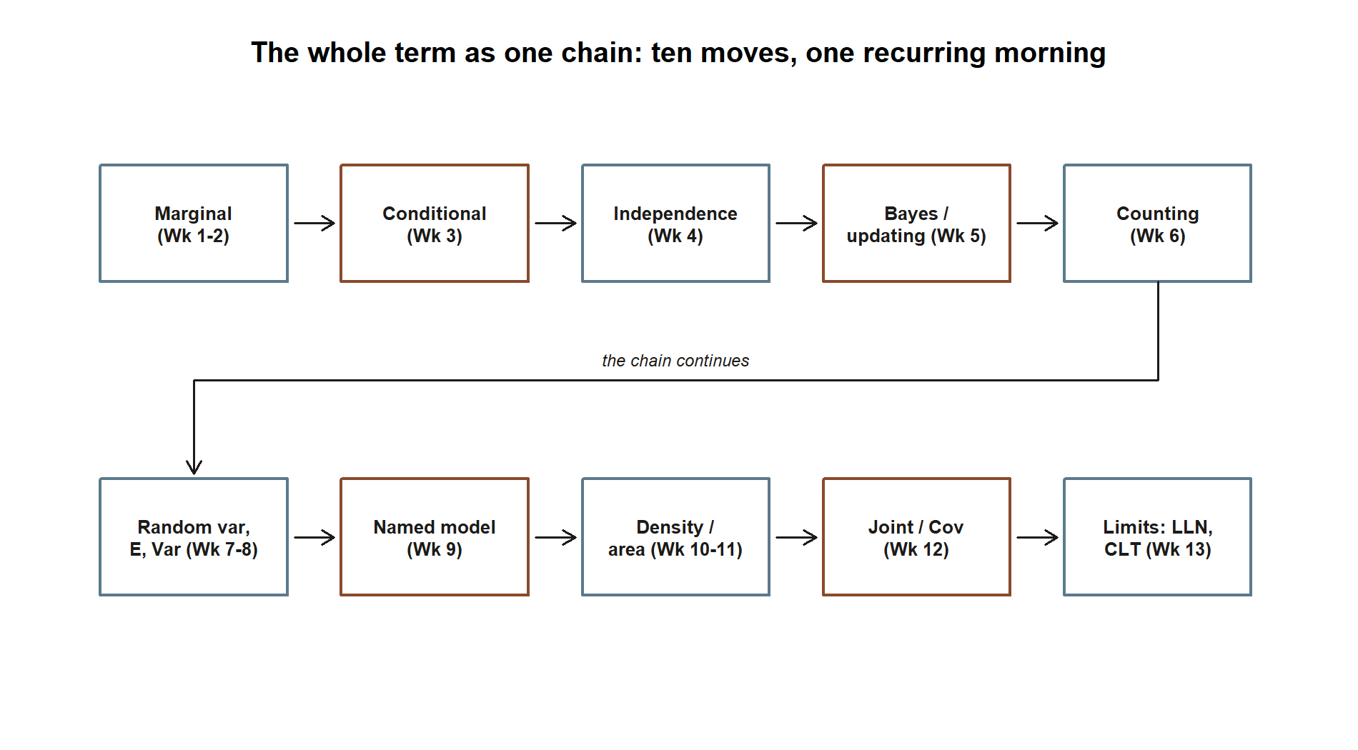
Here is the whole term as a single walk through Maya’s morning. Read it slowly; each arrow is a week.

It starts with uncertainty and a marginal. There is a \(0.30\) chance of rain, the shuttle is more reliable when it is dry, and combining those gives the headline number \(P(\text{on time}) = 0.81\), so \(P(\text{late}) = 0.19\). That single number was the whole point of Weeks 1–2: a probability is a summary of a described random world.

Then Maya learns something and we condition. Looking out the window changes the problem: \(P(\text{on time} \mid \text{rain}) = 0.60\), not \(0.81\). Conditioning is just restricting the world to the cases where what you learned is true (Week 3).

That immediately raises independence: is “on time” unaffected by “rain”? No — \(0.60 \ne 0.81\), so the two are dependent, which is exactly what makes the morning interesting. A fair coin flip on the side would be independent; the shuttle is not (Week 4).

Dependence makes updating possible. If Maya only learns she was late, she can run the arrow backward with Bayes’ rule and ask how likely rain was: \(P(\text{rain} \mid \text{late}) \approx 0.632\). The same machinery, applied to a medical screening test, produces the term’s most memorable surprise — a positive test for a rare condition still leaves the posterior near \(0.162\), because base rates dominate (Week 5).

To handle questions with many equally likely arrangements, we needed counting: a 10-question true/false quiz has \(2^{10} = 1024\) possible answer keys, and \(\binom{10}{k}\) of them have exactly \(k\) correct (Week 6).

Counting turned the quiz into a random variable \(X\) = number correct, with a pmf, and then a center and spread: \(E[X] = 5\), \(\operatorname{Var}(X) = 2.5\), \(\sigma \approx 1.58\) (Weeks 7–8).

That random variable had a name. \(X \sim \text{Binomial}(10, 0.5)\), and the arrivals at Maya’s stop are \(\text{Poisson}(4)\) per hour — named discrete models carry their mean, variance, and pmf with them (Week 9).

Asking how long she waits, rather than how many arrive, pushed us into the continuous world, where probability is area under a density: the wait is \(\text{Exponential}\) with mean \(15\) minutes, and her commute time is \(\text{Normal}(22, 5)\) with \(P(C \le 30) \approx 0.945\) (Weeks 10–11).

Two of these quantities move together, so we built a joint distribution for (rain, late) and measured the dependence we first spotted in Week 4 as a number: \(\operatorname{Cov} = 0.063\), \(\rho \approx 0.35\) (Week 12).

Finally, averaging many days of commute brought the limit theorems: the sample mean settles toward the true mean \(22\) (LLN), and the average of \(n\) days is approximately \(\text{Normal}(22, 5/\sqrt{n})\) (CLT, Week 13).

That is the entire course in one paragraph-per-week. Every formula you learned was one link in this chain. Seeing the whole chain as a single picture makes the “one link at a time” claim concrete:

Figure 1: The whole term as one chain (synthetic recap diagram). Ten moves, read left to right and wrapping down: marginal, conditional, independence, Bayes/updating, and counting across the top; random variable/expectation/variance, named model, density/area, joint/covariance, and the limit theorems across the bottom. Each arrow is a week.

What the figure shows (non-visual equivalent). Ten labeled boxes in reading order: Marginal (Wk 1–2), Conditional (Wk 3), Independence (Wk 4), Bayes/updating (Wk 5), Counting (Wk 6), Random variable/expectation/ variance (Wk 7–8), Named model (Wk 9), Density/area (Wk 10–11), Joint/covariance (Wk 12), Limits: LLN and CLT (Wk 13). An arrow connects each box to the next, including the wrap from Counting down to Random variable — the same order the paragraphs above just walked. Synthetic instructional example; numbers are illustrative.

The term’s load-bearing numbers (and what they mean)

A final rewards understanding the key numbers, not just listing them. Here are the term’s anchors with their meaning attached, in the same order as the chain above — read the table as a ladder, each row one rung past the row before it. All are synthetic; seed 35003 is set for any simulation.

Table 1: The term’s load-bearing numbers and what they mean, in the same order as the chain above – the numeric companion to the course-map diagram above.

Number	Where	What it means
\(0.81 \,/\, 0.19\)	Wk 1–2	overall chance the shuttle is on time / late, before you look outside
\(0.60\)	Wk 3	on-time chance given it is raining — conditioning lowers it from \(0.81\)
not independent	Wk 4	\(0.60 \ne 0.81\), so rain and lateness carry information about each other
\(0.632\)	Wk 5	\(P(\text{rain} \mid \text{late})\) — updating backward from effect to cause
\(0.162\)	Wk 5	screening posterior \(P(D \mid +)\) — a rare base rate survives a positive test
\(1024,\ \binom{10}{k}\)	Wk 6	total answer keys and the count with exactly \(k\) correct
\(E = 5,\ \operatorname{Var} = 2.5\)	Wk 7–8	center and spread of the guessed quiz score
\(\text{Poisson}(4)\)	Wk 9	arrivals per hour; mean \(=\) variance \(= 4\)
mean \(15\) min	Wk 11	exponential wait for the next shuttle
\(0.945\)	Wk 11	\(P(C \le 30)\) for a \(\text{Normal}(22, 5)\) commute
\(0.063,\ \rho \approx 0.35\)	Wk 12	covariance and correlation of rain and lateness — Week 4’s “dependent,” now numeric
\(\to 22\)	Wk 13	the long-run average commute the LLN drives toward

If you can say the meaning column out loud for each row, you understand the course. The equals signs are the easy part.

How to read a probability problem (the checklist)

The single most transferable thing this course can hand you is a way to start any problem. Four steps, in order:

1. Model. Name the objects. Is each quantity an event or a random variable? Discrete or continuous? What sample space, or what distribution? Write the assumptions down — independence, a fixed number of trials, a steady rate — before you compute. Most wrong answers are wrong here, not in the arithmetic.
2. Calculate. Now reach for the matching formula: an addition or multiplication rule, a conditional ratio, Bayes’ rule, a pmf or density, an expectation sum or integral, a named model’s mean and variance, or a limit theorem. The model from Step 1 tells you which one.
3. Interpret. Translate the number back into the world. “About \(5.5\%\)” or “the posterior is only \(0.162\)” — say what it means for Maya, the patient, or the manuscript. A probability with no interpretation is half an answer.
4. Check assumptions. Ask whether the model you assumed is actually plausible. Are the trials really independent? Is the rate really steady? Does a Poisson’s mean-equals-variance hold in the data? If the assumptions fail, the clean number is meaningless, and recognizing that is itself a correct answer.

Figure 2: The four-step checklist, as a loop (synthetic diagram). Model, calculate, interpret, check assumptions — read left to right. The dashed return arrow shows what happens when Step 4 turns up trouble: you revisit Step 1, not the arithmetic.

What the figure shows (non-visual equivalent). Four boxes in a row — Model, Calculate, Interpret, Check assumptions — each connected to the next by an arrow. A dashed arrow loops from the fourth box back to the first, labeled “if assumptions fail, revisit the model,” showing that a failed assumptions check sends you back to naming the objects, not back to redoing the arithmetic. Both worked examples below use these same four labels, in this order. Synthetic instructional example; numbers are illustrative.

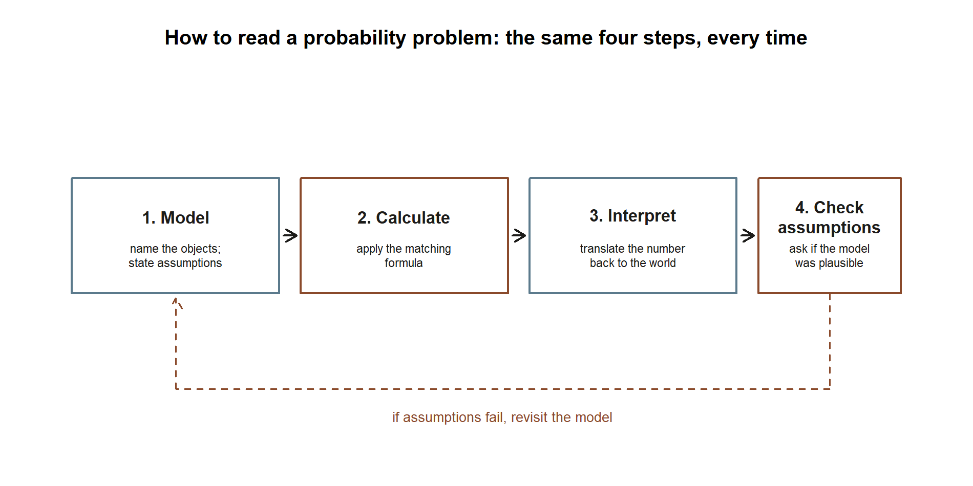
This is the same arc every concept week followed — describe, compute, interpret, sanity-check — compressed into four words you can carry into the exam: model, calculate, interpret, check.

Worked examples

This is a synthesis week, so we add no new transfer scenario — we re-walk the recurring slice and show the checklist running on it. All numbers are synthetic; seed 35003 set.

Worked example — one question, four moves on the recurring thread

Take a single composite question about Maya’s morning and watch the checklist sort it. “Maya was late this morning. How surprised should she be, and how does that revise her guess that it rained?”

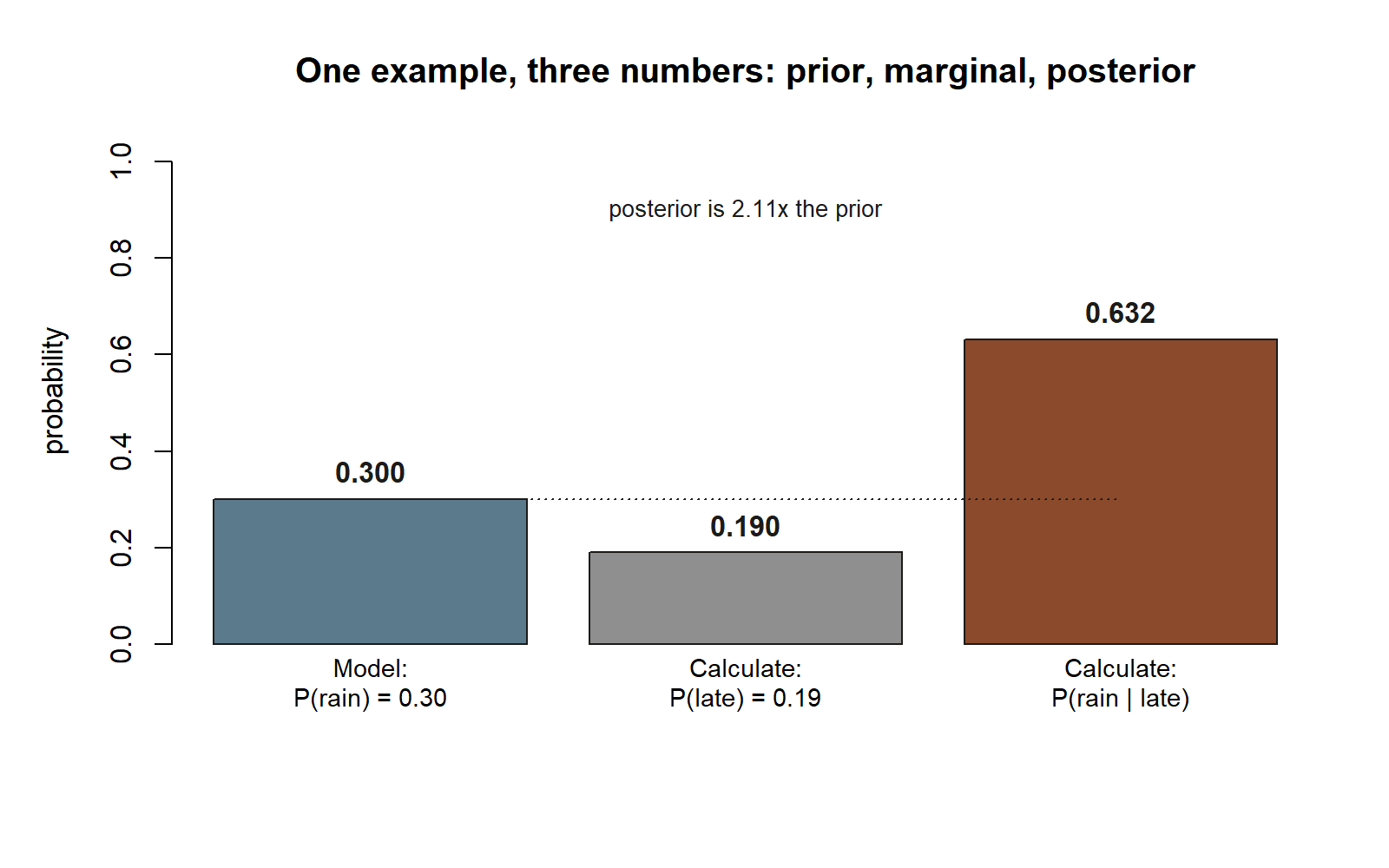
Model. “Late” and “rain” are events, not random variables, so this is a conditioning-and-updating problem, not a distribution problem. We have the marginals and the conditionals from the term: \(P(\text{rain}) = 0.30\), \(P(\text{late} \mid \text{rain}) = 0.40\), \(P(\text{late} \mid \text{no rain}) = 0.10\). The move is Bayes’ rule.

Calculate. First the marginal chance of being late, by the law of total probability:

\[ P(\text{late}) = P(\text{late} \mid \text{rain})P(\text{rain}) + P(\text{late} \mid \text{no rain})P(\text{no rain}) = 0.40(0.30) + 0.10(0.70) = 0.19. \]

Then run the arrow backward with Bayes’ rule:

\[ P(\text{rain} \mid \text{late}) = \frac{P(\text{late} \mid \text{rain})\,P(\text{rain})}{P(\text{late})} = \frac{0.40 \times 0.30}{0.19} = \frac{0.12}{0.19} \approx 0.632. \]

Interpret. Being late is a \(0.19\) event — uncommon but not rare, so it is mild evidence. Learning she was late lifts the chance it rained from the prior \(0.30\) up to about \(0.632\) — better than even, because lateness is much more likely on rainy mornings, but not a certainty, because dry mornings still occasionally run late.

Figure 3: One example, three numbers (synthetic). The Model step’s prior \(P(\text{rain})=0.30\), the Calculate step’s marginal \(P(\text{late})=0.19\), and the Calculate step’s posterior \(P(\text{rain}\mid\text{late})\approx 0.632\) — the checklist’s first two steps, read off as one chain of bars.

What the figure shows (non-visual equivalent). Three bars on the same \(0\)-to-\(1\) probability scale: the Model step’s prior \(P(\text{rain})=0.30\), the Calculate step’s marginal \(P(\text{late})=0.19\), and the Calculate step’s posterior \(P(\text{rain}\mid\text{late})\approx 0.632\). A dotted line at the prior’s height shows the posterior bar rising to a bit more than double it — the same numbers this worked example already derived, now shown as one chain instead of three separate lines of algebra. Synthetic instructional example; numbers are illustrative.

Check assumptions. The whole calculation rests on those two conditional rates (\(0.40\) and \(0.10\)) being stable, and on rain being the only relevant cause of lateness. If a road closure or a missed alarm were also in play, the model would be incomplete and the tidy \(0.632\) would overstate the rain’s role. Naming that limit is part of the answer.

That is the entire reading skill in one example: the four steps did the work, and the formula appeared only once we knew it was a Bayes problem.

Worked example — the same morning as a random variable and a joint pair

The recurring thread also lives on the random-variable side, and a final may ask it that way. Code rain as \(X\) (\(1\) if rain, \(0\) if not) and late as \(Y\) (\(1\) if late, \(0\) if not). The joint pmf we built in Week 12 is \(P(1,1) = 0.12\), \(P(1,0) = 0.18\), \(P(0,1) = 0.07\), \(P(0,0) = 0.63\).

Symbolic. Covariance measures how the two move together,

\[ \operatorname{Cov}(X, Y) = E[XY] - E[X]\,E[Y], \qquad \rho = \frac{\operatorname{Cov}(X, Y)}{\sigma_X \, \sigma_Y}. \]

Numeric. With \(E[X] = 0.30\), \(E[Y] = 0.19\), and \(E[XY] = P(1,1) = 0.12\),

\[ \operatorname{Cov}(X, Y) = 0.12 - 0.30(0.19) = 0.063, \qquad \rho \approx \frac{0.063}{0.1798} \approx 0.35. \]

Figure 4: The joint pmf, drawn (synthetic). The four joint probabilities as a shaded \(2\times2\) grid, darker meaning more probable; row and column totals are the marginals. The \((\text{rain}=1,\text{late}=1)\) cell, \(0.12\), is more than double the \(0.057\) an independent world would give it — dependence, made visible.

What the figure shows (non-visual equivalent). A \(2\times2\) grid of the joint pmf: \(P(1,1)=0.12\), \(P(1,0)=0.18\), \(P(0,1)=0.07\), \(P(0,0)=0.63\), with row totals \(0.30/0.70\) and column totals \(0.81/0.19\) matching the marginals. Darker shading marks a larger probability, so the \((0,0)\) cell (no rain, on time) is darkest. The \((1,1)\) cell, \(0.12\), is called out against the \(0.057\) an independent world would produce (\(P(\text{rain})\times P(\text{late}) = 0.30 \times 0.19\)) — the joint pmf puts more than double the independent weight on “rain and late together,” the numeric fingerprint of the positive covariance computed above. Synthetic instructional example; numbers are illustrative.

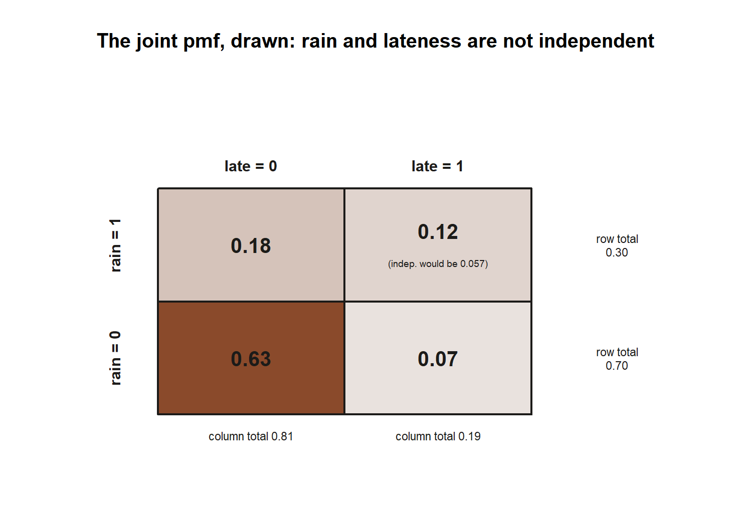
Interpret. The positive covariance is the number behind Week 4’s word “dependent”: rain and lateness go up together. And the consistency check ties the two halves of the course shut — from the joint pmf, \(P(\text{late} \mid \text{rain}) = 0.12 / 0.30 = 0.40\), exactly the conditional rate that drove the Bayes calculation above. The event view and the random-variable view are the same world described twice.

A common mistake

The signature synthesis-week error is reaching for a formula before naming the object — the exact thing the checklist exists to prevent. Under exam pressure it is tempting to scan a problem for numbers and start multiplying. That is how a marginal gets used where a conditional is needed, how a density value gets read as a probability, or how the binomial gets fitted to a “wait until the first success” story that is really geometric. None of these show up as arithmetic errors; the numbers look fine. They are modeling errors, and they are caught only in Step 1.

Figure 5: Two paths through the same problem (synthetic diagram). The top path skips straight to arithmetic and answers the wrong question with clean-looking numbers; the bottom path names the object first and answers the right question with the same arithmetic skill.

What the figure shows (non-visual equivalent). Two parallel two-box paths. Top (“wrong path”): “see numbers, start multiplying” leads to “clean arithmetic, wrong question answered.” Bottom (“right path”): “name the object: event or RV? which move?” leads to “matching formula, right question answered.” Both paths use the same arithmetic skill; only the first move differs, and that first move is exactly Step 1 of the checklist above. Synthetic instructional example; numbers are illustrative.

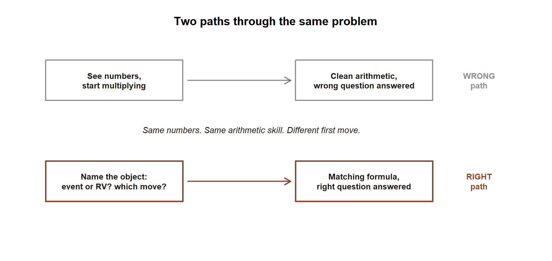
A second, related slip is forgetting to interpret and sanity-check. A bare number — “\(0.162\)” — is not a finished answer; the finished answer is “even after a positive test, the condition is still unlikely, because it is rare to begin with.” And a number built on a broken assumption (independent trials that are actually correlated, a steady rate that actually clusters) is worse than no number, because it looks authoritative. The fix for both is the same discipline you practiced all term: model first, then calculate, then say what it means, then ask whether you believe the model. Slow down at Steps 1 and 4 and the middle takes care of itself.

Low-stakes self-checks (ungraded)

These are for your own review — nothing here is collected or graded. Try to name the move before you compute.

1. Walk Maya’s morning from \(P(\text{on time}) = 0.81\) all the way to the CLT, naming the week and the probability idea at each link, without looking at the thread above.
2. For each, say which move it is — marginal, conditional, Bayes, counting, expectation, named model, density/area, joint, or a limit theorem: (a) \(P(\text{shuttle on time})\); (b) \(P(\text{rain} \mid \text{late})\); (c) \(P(C \le 30)\) for the commute; (d) \(\rho\) between rain and lateness; (e) the average of \(50\) commutes.
3. Recompute \(P(\text{rain} \mid \text{late}) \approx 0.632\) from \(P(\text{rain}) = 0.30\), \(P(\text{late} \mid \text{rain}) = 0.40\), \(P(\text{late} \mid \text{no rain}) = 0.10\), and explain in one sentence why the posterior rose above the prior.
4. State what each anchor number means (not just equals): \(0.945\), \(0.162\), \(E[X] = 5\), \(\rho \approx 0.35\), and “\(\to 22\).”
5. Pick any problem from any earlier week, and write the four checklist steps for it — model, calculate, interpret, check assumptions — in full sentences.

Reading and source pointer

This is a review week, so point yourself at both course texts and skim broadly rather than deeply. For a chapter-by-chapter re-walk of the whole term’s spine — sample spaces and rules, conditional probability and Bayes, counting, random variables, the standard discrete and continuous models, joint distributions, and the limit theorems — return to Grinstead & Snell, reading the chapter that matches each week of the arc: https://www.dartmouth.edu/~chance/teaching_aids/books_articles/probability_book/book.html.

For a second source of review and practice in a different voice, use the MIT OpenCourseWare 18.05 review materials and practice problems; working a few of its problems alongside your re-walk is a good way to test whether the reading skill transfers off the commuter thread: https://ocw.mit.edu/courses/18-05-introduction-to-probability-and-statistics-spring-2022/.

These notes are the course’s own synthesis, grounded in but not copied from the sources.

Public vs. graded

These notes, the examples, and the practice here are public and ungraded — study material only. No graded prompts, answer keys, rubrics, point values, or due dates appear on this site. Graded checkpoints, quizzes, homework, labs, the midterm, the project, and the final live in Blackboard (the LMS), which is authoritative for due dates, submissions, and grades. If this page and Blackboard ever disagree, follow Blackboard.

Looking ahead

The last class meets Monday, December 7; a consultation day follows, and the cumulative final lands in the end-of-term window (the exact block is posted in Blackboard, which is authoritative — no date or block is fixed on this page). What is “ahead” is really what is next after this course: every move you practiced here is the foundation under statistical inference. The conditioning and updating of Week 5 grow into Bayesian statistics; the expectation, variance, and named models become the building blocks of estimators; and the limit theorems of Week 13 are the reason a sample mean can stand in for a population mean at all. You leave with a reading skill — model, calculate, interpret, check — that outlasts every formula on the final.

See also

• Course syllabus — the full schedule and where graded work, including the final, lives (Blackboard is authoritative for all dates and the exam block).
• Notation glossary — every symbol and model parameterization the term used, in one place — the right thing to skim before the final.
• Distribution reference — a one-stop table of each named model’s pmf or density, mean, variance, and support, for the Week 9 and Week 11 strands.
• Review aids — the four simulation labs, each re-checking a piece of the thread by simulation: Lab 2: Monte Carlo basics, Lab 5: Bayes by simulation, Lab 9: Simulating discrete models, and Lab 13: Law of large numbers and the CLT.
• Week 1 — Uncertainty, probability & models — the start of the thread, where \(P(\text{on time}) = 0.81\) first appeared.
• Week 5 — Bayes’ rule & updating — the updating move at the heart of the recurring slice above.
• Week 13 — Sums, simulation & limit behavior — the final link in the chain, where averages settle toward \(22\).
• Week 14 — Probability modeling project — the project that put the whole arc to work just before this review.