set.seed(35003)
# All 36 equally likely ordered outcomes of two fair dice.
grid <- expand.grid(first = 1:6, second = 1:6)
p <- 1 / nrow(grid)                       # each outcome has probability 1/36

A  <- grid$first == 1                      # event A: first die = 1
D7 <- (grid$first + grid$second) == 7      # event D: sum = 7
D2 <- (grid$first + grid$second) == 2      # event D': sum = 2

# Compare P(A and D) with P(A) * P(D) for each total.
joint7 <- p * sum(A & D7); prod7 <- (p * sum(A)) * (p * sum(D7))
joint2 <- p * sum(A & D2); prod2 <- (p * sum(A)) * (p * sum(D2))

c(joint7 = joint7, prod7 = prod7)          # equal  -> independent for sum = 7
c(joint2 = joint2, prod2 = prod2)          # unequal -> dependent for sum = 2

# The same comparison, restated as CONDITIONAL probabilities (a second view of the same numbers),
# plus a shown-not-run plot -- run this yourself to reproduce the bar chart shown just below.
p_D7_given_A <- joint7 / (p * sum(A))      # P(sum = 7 | first = 1)
p_D7         <- p * sum(D7)                # P(sum = 7)
p_D2_given_A <- joint2 / (p * sum(A))      # P(sum = 2 | first = 1)
p_D2         <- p * sum(D2)                # P(sum = 2)

par(mfrow = c(1, 2))
barplot(c(p_D7_given_A, p_D7), names.arg = c("P(sum=7|first=1)", "P(sum=7)"),
        main = "Sum = 7: bars match (independent)")
barplot(c(p_D2_given_A, p_D2), names.arg = c("P(sum=2|first=1)", "P(sum=2)"),
main = "Sum = 2: bars differ (dependent)")Week 4 — Independence & information
When knowing one event tells you nothing about another
The week question
Last week we learned to update: once we learn that an event \(B\) has occurred, the conditional probability \(P(A\mid B)\) tells us how likely \(A\) is in that smaller, reweighted world. The natural next question is the one this week answers: are there pairs of events where learning \(B\) changes nothing?
That is the whole idea of independence. Two events are independent when knowing that one happened leaves your probability for the other exactly where it started — no nudge up, no nudge down. The week question is therefore simple to state and surprisingly easy to get wrong: when does one event carry information about another, and when does it carry none at all?
Why this matters
Independence is the hinge on which most of the rest of the course turns. Almost every formula you will meet later — the binomial counting in Week 9, the variance-of-a-sum bookkeeping in Week 12, the law of large numbers and the central limit theorem in Week 13 — quietly assumes that certain events or measurements are independent. When that assumption holds, probabilities multiply, and a hard joint question collapses into a product of easy ones. When it fails, the same multiplication gives a confidently wrong answer.
So independence is doing two jobs at once. It is a modeling assumption — a claim about the world that you choose to make and should be ready to defend — and it is a computational shortcut that only earns its keep when the assumption is true. A large part of becoming fluent in probability is learning to tell the difference between “these events have nothing to do with each other” and “I would like them to have nothing to do with each other because it makes my arithmetic easier.”
This week also clears up the single most common confusion in a first probability course: independence is not the same thing as two events not being able to happen together. Those are opposite phenomena, and we will see exactly why.
Learning goals
By the end of this week you should be able to:
- State the definition of independence three equivalent ways: as a product rule \(P(A\cap B)=P(A)\,P(B)\), and as the two “no information” conditions \(P(A\mid B)=P(A)\) and \(P(B\mid A)=P(B)\).
- Decide whether two specific events are independent by checking the product rule directly, rather than by intuition.
- Explain why “on time” and “rain” in our commuter world are not independent, using the actual numbers.
- Explain why two flips of a fair coin are independent.
- Distinguish independence from mutual exclusivity, and explain why two disjoint events of positive probability are necessarily dependent.
- Recognize when independence is a reasonable physical assumption and when it must instead be checked against probabilities.
Core vocabulary
- Independent events \(A \perp B\) — two events such that the occurrence of one does not change the probability of the other. Formally, \(A\) and \(B\) are independent when \(P(A\cap B)=P(A)\,P(B)\).
- Dependent events — any pair that is not independent; learning one shifts the probability of the other, in either direction.
- Product rule (for independent events) — the statement \(P(A\cap B)=P(A)\,P(B)\). It is a definition of independence, not a law that always holds; it holds exactly when the events are independent.
- General multiplication rule — the always-true statement \(P(A\cap B)=P(A\mid B)\,P(B)\) from Week 3. It holds for every pair with \(P(B)>0\). Independence is the special case where \(P(A\mid B)\) simplifies to \(P(A)\).
- Mutually exclusive (disjoint) events — events that cannot both occur, so \(A\cap B=\varnothing\) and \(P(A\cap B)=0\). This is a statement about overlap, and it is not independence.
- Information — used informally here: \(B\) “carries information about” \(A\) when \(P(A\mid B)\neq P(A)\). Independence is precisely the case of no information.
Concept development
From conditioning to independence
Week 3 gave us the general multiplication rule, which is always true whenever the conditioning event has positive probability:
\[ P(A\cap B)=P(A\mid B)\,P(B), \qquad P(B)>0. \]
This says nothing special yet — it is just the definition of conditional probability rearranged. The interesting question is what happens for the special pairs where conditioning on \(B\) does not move the probability of \(A\). Suppose
\[ P(A\mid B)=P(A). \]
In words: learning that \(B\) happened leaves your probability for \(A\) unchanged. Substitute this into the multiplication rule and the conditional collapses into the plain marginal:
\[ P(A\cap B)=P(A\mid B)\,P(B)=P(A)\,P(B). \]
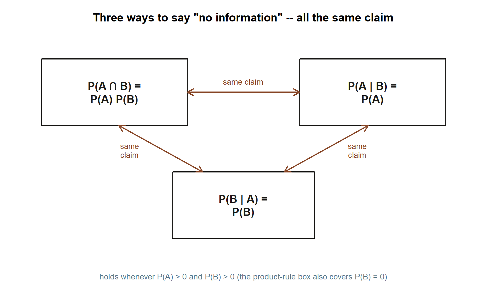
That product form, \(P(A\cap B)=P(A)\,P(B)\), is the official definition of independence, written \(A \perp B\). It is the cleaner definition for two reasons. First, it is symmetric — it treats \(A\) and \(B\) the same way, so independence is automatically a two-way street: if \(B\) tells you nothing about \(A\), then \(A\) tells you nothing about \(B\). Second, it makes sense even when \(P(B)=0\), where the conditional \(P(A\mid B)\) is undefined. For events with positive probability, all three statements below say exactly the same thing:
\[ A \perp B \iff P(A\cap B)=P(A)\,P(B) \iff P(A\mid B)=P(A) \iff P(B\mid A)=P(B). \]
The practical takeaway: to decide whether two events are independent, you usually check the product rule, because it only needs three numbers — \(P(A)\), \(P(B)\), and \(P(A\cap B)\) — and never asks you to compute a conditional probability.
Independence as a modeling assumption versus a fact to be checked
There are two very different situations in practice, and keeping them apart is most of the skill.
Sometimes independence is a physical assumption you make up front because the mechanism guarantees it. A fair coin has no memory: the second flip does not consult the first. Two cards drawn from separate, freshly shuffled decks do not influence each other. In these cases you assert independence from how the world works, and then you are allowed to multiply. This is the normal way independence enters a model.
Other times you are handed a full probability description — a table, a tree, or a set of conditional probabilities — and independence becomes a fact to be verified, not assumed. You check whether \(P(A\cap B)\) really equals \(P(A)\,P(B)\). The answer is whatever the numbers say, regardless of whether the events “feel” related. Our commuter world is exactly this second kind of situation: we already specified all the probabilities back in Weeks 1 through 3, so independence here is not up for negotiation — it is settled by arithmetic.
The danger is sliding from the first mode into the second by habit: assuming independence (because it makes the multiplication easy) for events that the numbers say are dependent. That is the single most common way a probability calculation goes silently wrong.
Independence is not mutual exclusivity
These two ideas are constantly confused because both involve a pair of events and both feel like the events are “separate.” They are in fact opposites.
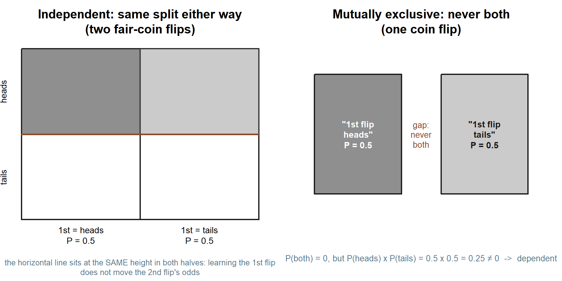
Mutually exclusive means the events cannot both happen: their intersection is empty, so \(P(A\cap B)=0\). Knowing that one occurred tells you the other definitely did not. That is the strongest possible information one event can carry about another — it is the opposite of “no information.”
Independent means \(P(A\cap B)=P(A)\,P(B)\): knowing one occurred tells you nothing about the other.
Now put the two together. Suppose \(A\) and \(B\) are mutually exclusive and both have positive probability, \(P(A)>0\) and \(P(B)>0\). Then
\[ P(A\cap B)=0 \quad\text{but}\quad P(A)\,P(B)>0, \]
so \(P(A\cap B)\neq P(A)\,P(B)\), and the events are dependent. The logic is intuitive once you see it: if \(A\) and \(B\) cannot coexist, then learning \(A\) happened drives the probability of \(B\) all the way down to zero — a very large amount of information. Two disjoint events of positive probability are therefore necessarily dependent, never independent. The only way an event can be both mutually exclusive with \(A\) and independent of \(A\) is if it has probability zero, which is a degenerate edge case, not a useful model.
Keep the slogan in mind for the rest of the course: disjoint is a statement about overlap; independent is a statement about information. They are different questions with, usually, opposite answers.
Worked examples
We work each example symbolically first — writing the independence check as a comparison of two quantities — and then plug in numbers. All data are synthetic; seed 35003 set.
Worked example — the commuter slice: is “on time” independent of “rain”?
Recall Maya’s morning shuttle. The fixed probabilities are \(P(\text{rain})=0.30\), with the shuttle’s reliability depending on the weather: \(P(\text{on time}\mid\text{rain})=0.60\) and \(P(\text{on time}\mid\text{no rain})=0.90\). Combining these (the total-probability calculation from Week 3) gave the marginal
\[ P(\text{on time})=0.60(0.30)+0.90(0.70)=0.81. \]
Let \(A=\{\text{on time}\}\) and \(B=\{\text{rain}\}\). Symbolically, \(A\) and \(B\) are independent if and only if \(P(A\mid B)=P(A)\) — that is, if and only if the on-time rate on rainy days equals the on-time rate overall. Numerically, those two numbers are
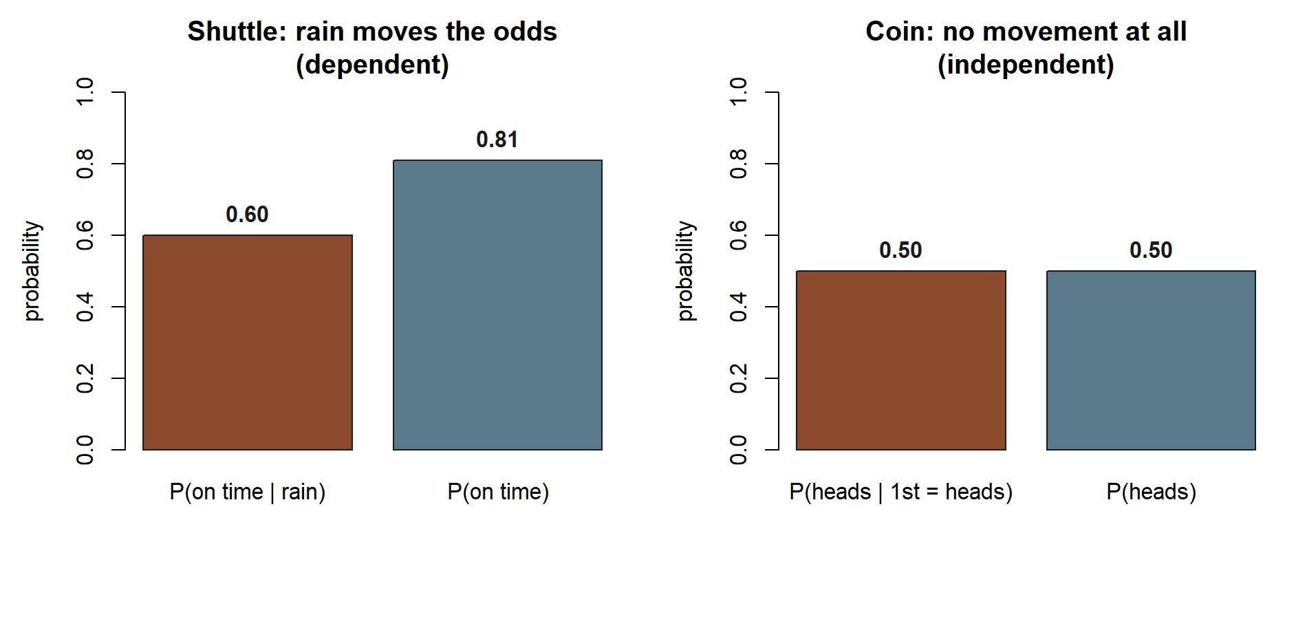
\[ P(\text{on time}\mid\text{rain})=0.60 \qquad\text{versus}\qquad P(\text{on time})=0.81. \]
Since \(0.60 \neq 0.81\), the events are not independent. We can confirm with the product-rule form. The joint probability of a rainy, on-time morning is
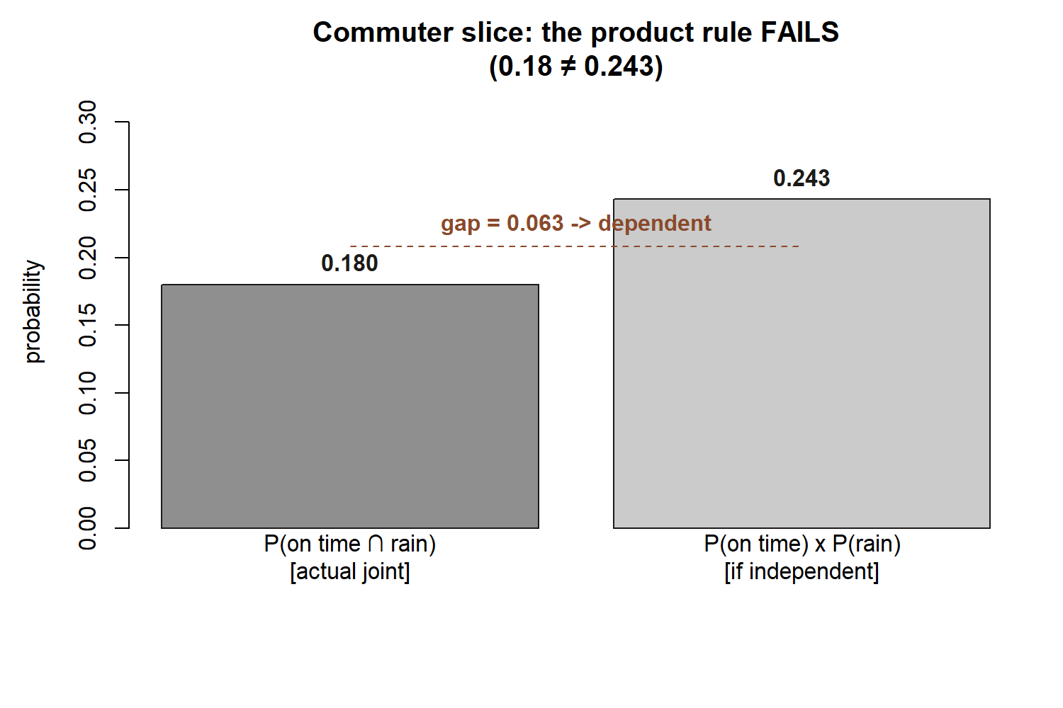
\[ P(\text{on time}\cap\text{rain})=P(\text{on time}\mid\text{rain})\,P(\text{rain})=0.60(0.30)=0.18, \]
while the product of the marginals is
\[ P(\text{on time})\,P(\text{rain})=0.81(0.30)=0.243. \]
Because \(0.18 \neq 0.243\), the product rule fails, and “on time” and “rain” are dependent — exactly the same verdict we reached from the conditional. And the direction makes sense: rain lowers the chance of an on-time shuttle (\(0.60 < 0.81\)), so rain carries genuine information. This dependence is the seed of the positive correlation between rain and lateness we will quantify in Week 12.
Worked example — two flips of a fair coin (independent by construction)
Now a case that goes the other way. Flip a fair coin twice and record each result. Let \(A=\{\text{first flip is heads}\}\) and \(B=\{\text{second flip is heads}\}\). A fair coin has no memory, so we model the two flips as independent — this is an assumption justified by the physics, not something forced on us by a table.
Symbolically, independence means \(P(A\cap B)=P(A)\,P(B)\). The four equally likely outcomes of two flips are HH, HT, TH, TT, each with probability \(\tfrac14\). Numerically, \(P(A)=\tfrac12\) (the first flip is heads in HH and HT) and \(P(B)=\tfrac12\) (the second flip is heads in HH and TH), while the only outcome with both flips heads is HH, so
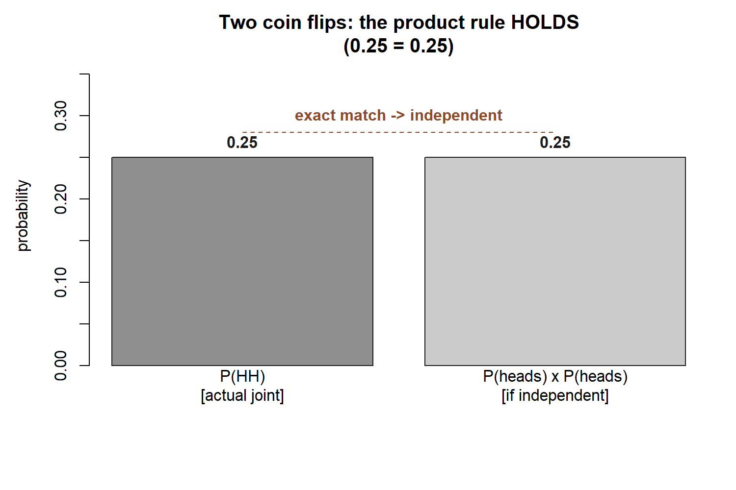
\[ P(A\cap B)=P(\text{HH})=\tfrac14 \qquad\text{and}\qquad P(A)\,P(B)=\tfrac12\cdot\tfrac12=\tfrac14. \]
The two sides agree, so \(A \perp B\): the flips are independent, exactly as the no-memory model demands. Equivalently, \(P(B\mid A)=\tfrac14 / \tfrac12=\tfrac12=P(B)\) — learning the first flip was heads tells you nothing about the second. This is the clean opposite of the commuter case: there, conditioning moved the probability (\(0.60\) versus \(0.81\)); here, it leaves it untouched.
A quick check that disjointness is a different question: are “first flip heads” and “first flip tails” independent? They are mutually exclusive (a single flip cannot be both), each has probability \(\tfrac12 > 0\), so by the rule above they must be dependent — and indeed \(P(\text{both})=0 \neq \tfrac12\cdot\tfrac12=\tfrac14\). Mutual exclusivity, once again, is the opposite of independence.
Put the two worked examples above side by side and the whole week compresses into one picture: the same “conditional versus marginal” comparison, once with bars that move and once with bars that do not.
Worked example — transfer: two dice, and the trap of “sum = 7”
Take a new scene to test the idea. Roll two fair dice and look at the two face values. The 36 ordered outcomes \((i,j)\) are equally likely.
First, the two individual face values are independent, by construction: one die cannot influence the other. Let \(A=\{\text{first die}=1\}\) and \(C=\{\text{second die}=1\}\). Symbolically we check \(P(A\cap C)=P(A)\,P(C)\). Numerically, \(P(A)=\tfrac{6}{36}=\tfrac16\) and likewise \(P(C)=\tfrac16\), while only the single outcome \((1,1)\) puts both at one, so
\[ P(A\cap C)=\tfrac{1}{36} \qquad\text{and}\qquad P(A)\,P(C)=\tfrac16\cdot\tfrac16=\tfrac{1}{36}. \]
They match, so the two face values are independent — knowing the first die is a 1 says nothing about the second.
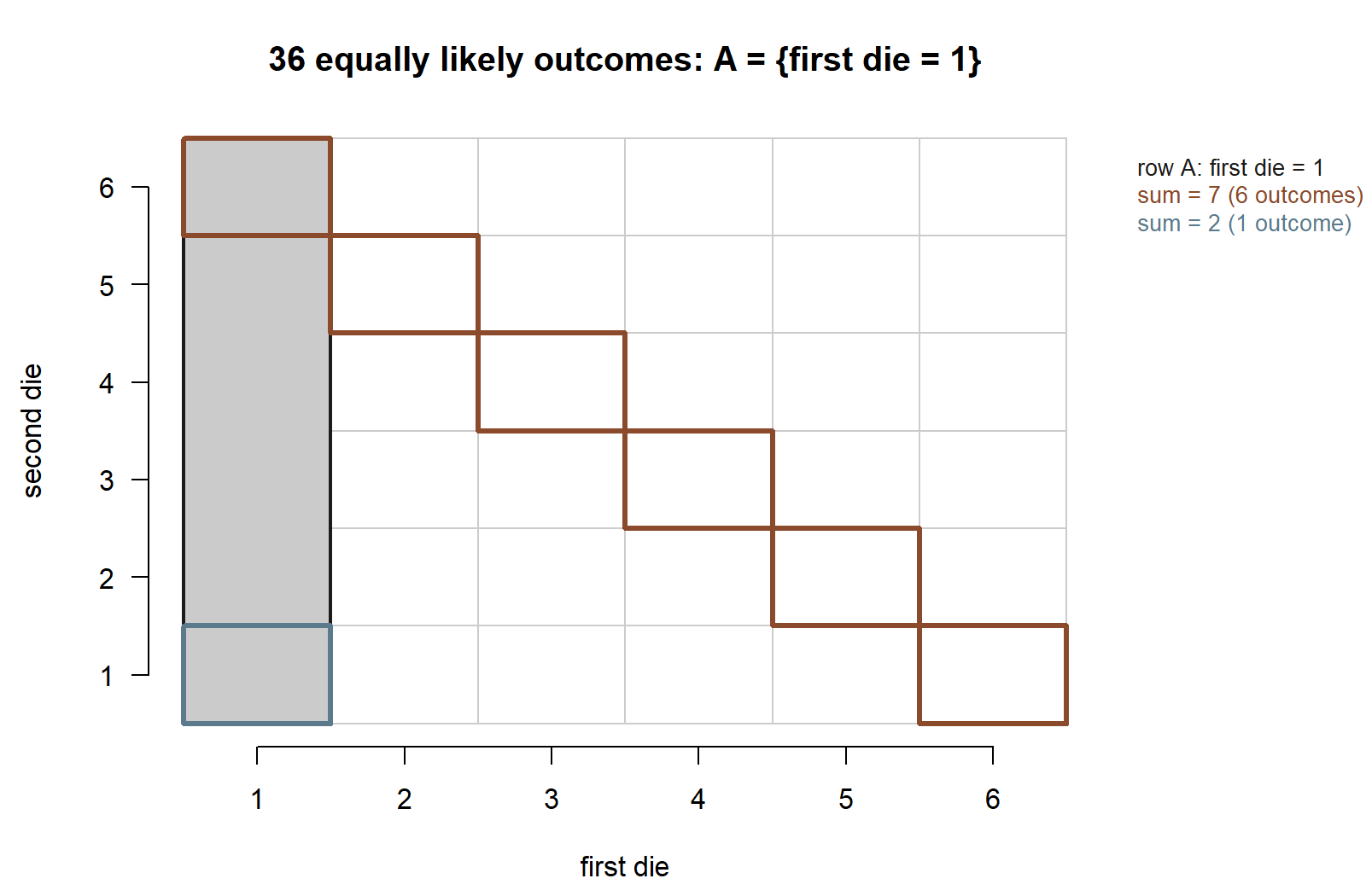
Now the trap. Let \(D=\{\text{the sum of the two dice}=7\}\) and keep \(A=\{\text{first die}=1\}\). It is tempting to assume \(A\) and \(D\) are independent because “the dice rolls are independent.” But the sum is a property of both dice at once, so conditioning on the first die can change what sums are reachable. Symbolically, check \(P(A\cap D)\) against \(P(A)\,P(D)\). The outcomes summing to 7 are \((1,6),(2,5),(3,4),(4,3),(5,2),(6,1)\) — six of them — so \(P(D)=\tfrac{6}{36}=\tfrac16\). The only outcome that is both “first die = 1” and “sum = 7” is \((1,6)\), so \(P(A\cap D)=\tfrac{1}{36}\). Compare:
\[ P(A\cap D)=\tfrac{1}{36} \qquad\text{and}\qquad P(A)\,P(D)=\tfrac16\cdot\tfrac16=\tfrac{1}{36}. \]
These two happen to be equal, so for the specific total 7, \(A=\{\text{first die}=1\}\) and \(D=\{\text{sum}=7\}\) are independent. The number 7 is special: because each face value \(1\) through \(6\) has exactly one partner that completes a sum of 7, fixing the first die never changes the chance the sum is 7.
The dependence appears the moment you pick a different total. Take \(D'=\{\text{sum}=2\}\). The only way to sum to 2 is \((1,1)\), so \(P(D')=\tfrac{1}{36}\), and the event “first die = 1 and sum = 2” is again just \((1,1)\), giving \(P(A\cap D')=\tfrac{1}{36}\). But
\[ P(A\cap D')=\tfrac{1}{36} \qquad\text{versus}\qquad P(A)\,P(D')=\tfrac16\cdot\tfrac{1}{36}=\tfrac{1}{216}, \]
and \(\tfrac{1}{36}\neq\tfrac{1}{216}\), so \(A\) and \(D'\) are dependent: learning the first die is a 1 raises the chance of a sum of 2 from \(\tfrac{1}{36}\) all the way to \(\tfrac16\) (you now only need the second die to be a 1). The lesson is the one this whole week is built around: the individual dice being independent does not make every event about them independent. You must check the actual events, with the actual product rule, rather than reasoning from the inputs.
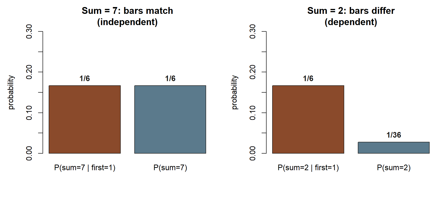
The same idea can be expressed as a short, shown-not-run R sketch — extended below with a plotting block that reproduces the bar chart just above. (In this build R is teaching code — displayed, not executed; run it yourself to reproduce.)
A common mistake
The mistake that costs the most points later is confusing independence with mutual exclusivity — and its close cousin, assuming independence to make the multiplication easy.
Students often reason: “These two events seem unrelated, so they can’t both happen, so I’ll treat them as independent.” Every step there is shaky. “Can’t both happen” is mutual exclusivity, which (for positive -probability events) forces \(P(A\cap B)=0\) and therefore makes the events dependent, the exact opposite of what was intended. And “seem unrelated” is intuition, not a check. The fix is mechanical and reliable: never declare independence from a feeling. Either you can name a physical reason the mechanism has no memory (separate fair coins, separate dice, freshly shuffled decks), in which case independence is a justified modeling assumption, or you have the numbers and verify \(P(A\cap B)=P(A)\,P(B)\) directly. If the product rule fails — as it does for “on time” and “rain,” where \(0.18\neq0.243\) — the events are dependent, and multiplying \(P(A)\,P(B)\) would give the wrong joint probability. When in doubt, fall back on the always-true general rule \(P(A\cap B)=P(A\mid B)\,P(B)\), which never assumes anything.
Low-stakes self-checks (ungraded)
These are for your own practice — ungraded, no submission. Try each before reading on.
- In the commuter world, you found \(P(\text{on time}\cap\text{rain})=0.18\) but \(P(\text{on time})\,P(\text{rain})=0.243\). Without recomputing, state in one sentence what the gap between these two numbers tells you about whether rain carries information about an on-time shuttle.
- Two flips of a fair coin gave \(P(A\cap B)=\tfrac14=P(A)\,P(B)\). Suppose instead the coin were bent so that \(P(\text{heads})=0.7\) on each independent flip. Predict \(P(\text{both heads})\) and check that the two flips are still independent.
- Explain, in your own words, why two events that are mutually exclusive and both have positive probability can never be independent. Use the two-flip example “first flip heads” versus “first flip tails.”
- For two fair dice, you saw that “first die = 1” and “sum = 7” are independent but “first die = 1” and “sum = 2” are not. Pick the total “sum = 6” and decide whether “first die = 1” and “sum = 6” are independent by checking the product rule. (Hint: how many ways sum to 6, and is \((1,5)\) one of them?)
- A student claims, “Independence means the two events can’t overlap.” Write a one-sentence correction that names the two ideas being confused.
Reading and source pointer
This week is grounded in the conditional-probability and independence material of the two course texts; read either or both alongside these notes.
- Grinstead & Snell, Introduction to Probability, Ch 4 (Conditional Probability) — develops conditional probability and the definition of independence, including the product-rule characterization and the contrast with events that cannot co-occur. Free online: https://www.dartmouth.edu/~chance/teaching_aids/books_articles/probability_book/book.html.
- MIT OpenCourseWare 18.05 (conditional probability, independence) — its conditional-probability and independence material reinforces the “no information” reading of independence and the base-rate intuition behind dependent events. Free at: https://ocw.mit.edu/courses/18-05-introduction-to-probability-and-statistics-spring-2022/.
These notes are the course’s own synthesis, grounded in but not copied from the sources. All example data are synthetic, with seed 35003 set.
Public vs. graded
These notes, the examples, and the practice here are public and ungraded — study material only. No graded prompts, answer keys, rubrics, point values, or due dates appear on this site. Graded checkpoints, quizzes, homework, labs, the midterm, the project, and the final live in Blackboard (the LMS), which is authoritative for due dates, submissions, and grades. If this page and Blackboard ever disagree, follow Blackboard.
Looking ahead
Independence told us when conditioning changes nothing. Next week we turn the spotlight back onto the cases where conditioning changes a lot, and we learn to run the conditioning backwards. In Week 5 — Bayes’ rule & updating we will start from \(P(\text{on time}\mid\text{rain})\) and recover the reverse direction \(P(\text{rain}\mid\text{late})\), and we will meet the headline example of the course — a medical screening test where a positive result is far less alarming than it first appears. The dependence we measured this week between rain and lateness is precisely what makes those reverse questions interesting: if the events were independent, there would be nothing to update.
See also
- Week 3 — Conditional probability — the multiplication rule and the \(0.60\)-versus-\(0.81\) slice this week builds on.
- Week 5 — Bayes’ rule & updating — running the conditioning backward once events are known to be dependent.
- Week 12 — Joint distributions & dependence — where the rain-and-lateness dependence becomes a covariance and a correlation.
- Notation glossary — the binding symbols, including \(A \perp B\) and \(P(A\mid B)\).
- Distribution reference — the standard models that will assume independence later in the course.
- Syllabus — course rhythm, policies, and where graded work lives.
Week 4 has no companion lab; the simulation strand resumes with the Week 5 Bayes-by-simulation lab.