Week 3 — Conditional probability

How a probability changes once you know something

The week question

Last week we assigned a probability to an event once the sample space and the rules were settled. That number is a before-you-know-anything statement. But real mornings are not like that: you wake up, you look out the window, and you learn something. The question this week is simple to state and surprisingly deep — once you know that some event has happened, how should the probability of everything else change?

Return to Maya, our commuter student, and her campus shuttle. Across the whole term she catches it on time about \(81\%\) of mornings; that is the marginal figure \(P(\text{on time}) = 0.81\) we built last week. But this morning it is raining. Should she still plan around \(0.81\)? The honest answer is no: when it rains, the shuttle runs on time only \(60\%\) of the time. The same shuttle, the same student — but the rain has changed what she should expect. The number \(0.60\) is a conditional probability, and learning to compute and reason with it is the whole job of Week 3.

A scheduling note: this is a compressed week. Labor Day falls on the Monday, so there is no Monday class — we meet Wednesday and Friday only. The development below is trimmed to the conditioning core (the definition, the multiplication rule, and the probability tree) so that two meetings are enough.

Why this matters

Conditional probability is the hinge on which the rest of this course turns. Almost everything interesting in probability is a statement about how one event’s chance shifts in light of another: a test result given a disease, a defect given a supplier, a late shuttle given the weather. If you can only ever quote the marginal probability — the long-run rate ignoring all context — you are throwing away exactly the information that makes a decision worth making.

It matters for three reasons you will feel all term. First, updating: conditioning is how a probability absorbs evidence, and Week 5’s Bayes’ rule is conditioning run in two directions at once. Second, independence: next week we ask when learning \(B\) leaves \(P(A)\) unchanged, a question that only makes sense once conditioning is in hand. Third, modeling: trees, joint distributions, and the standard models later in the term are all built by chaining conditional statements together.

Learning goals

By the end of this week you should be able to:

• State in plain language what \(P(A \mid B)\) means and why it can differ from \(P(A)\).
• Apply the definition \(P(A \mid B) = P(A \cap B) / P(B)\), and say why it requires \(P(B) > 0\).
• Rearrange the definition into the multiplication rule \(P(A \cap B) = P(A \mid B)\,P(B)\) and use it to find the probability of a joint event.
• Draw and read a probability tree for a two-stage process, multiplying along a path to get a path probability.
• Distinguish forward conditioning (cause \(\to\) effect, the direction we work this week) from the reverse direction we will need for Bayes in Week 5.

Core vocabulary

• Conditional probability \(P(A \mid B)\) — the probability of \(A\) given that \(B\) has occurred. Read the bar “\(\mid\)” as the word “given.” It is defined only when \(P(B) > 0\).
• Conditioning event — the thing we treat as known, written on the right of the bar (\(B\) above). To condition on \(B\) is to restrict attention to the worlds where \(B\) is true.
• Joint probability \(P(A \cap B)\) — the probability that \(A\) and \(B\) both happen.
• Multiplication rule — \(P(A \cap B) = P(A \mid B)\,P(B)\), the definition rearranged so we can build a joint probability from a conditional one.
• Probability tree — a branching diagram for a multi-stage experiment; each branch carries a conditional probability, and multiplying along a path gives that path’s probability.
• Forward conditioning — conditioning in the natural cause-to-effect direction (here, rain \(\to\) on time). The reverse direction (effect \(\to\) cause) waits for Bayes in Week 5.

Concept development

Restricting the world to “given B”

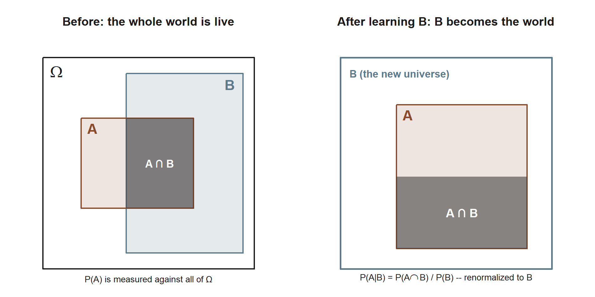
The cleanest way to picture conditioning is as a change of which outcomes are still in play. Before you know anything, the whole sample space \(\Omega\) is live and \(P(A)\) measures \(A\) against all of it. The moment you learn that \(B\) has occurred, every outcome outside \(B\) is ruled out — those worlds simply did not happen. So the new universe is \(B\) itself, and we ask: within \(B\), how much of it is also \(A\)? That overlap is \(A \cap B\) measured against \(B\), which as a fraction gives the definition:

\[ P(A \mid B) = \frac{P(A \cap B)}{P(B)}, \qquad P(B) > 0. \]

Two things to read off immediately. The denominator is \(P(B)\), not \(P(\Omega) = 1\) — we have renormalized to the smaller world \(B\). And the precondition \(P(B) > 0\) is not a technicality to skip: if \(B\) has probability zero, “given \(B\)” describes a world that never occurs, and the fraction divides by zero. Conditioning on an impossible event is undefined, full stop.

Figure 1: Restricting the world to “given B” (synthetic diagram). Left: before you know anything, \(A\) and \(B\) both sit inside the full sample space \(\Omega\), and \(P(A)\) is measured against all of it. Right: once you learn \(B\) has occurred, \(B\) itself becomes the new universe — the same overlap \(A \cap B\) is now measured against \(B\), which is exactly \(P(A \mid B) = P(A \cap B)/P(B)\).

What the figure shows (non-visual equivalent). Before conditioning, \(A\) and \(B\) are two regions inside the whole space \(\Omega\), and \(P(A)\) compares \(A\)’s area to all of \(\Omega\). After you learn \(B\) is true, every outcome outside \(B\) is discarded, so \(B\) becomes the whole universe; the conditional probability \(P(A \mid B)\) compares the same overlap \(A \cap B\) to the new, smaller universe \(B\) instead of to \(\Omega\). Synthetic diagram; illustrative.

The multiplication rule: building a joint from a conditional

The definition is often easier to use in a rearranged form. Multiply both sides by \(P(B)\):

\[ P(A \cap B) = P(A \mid B)\,P(B). \]

This is the multiplication rule (sometimes the “chain rule” for two events). It says you can build the probability of “\(A\) and \(B\)” by first asking how likely \(B\) is, then asking how likely \(A\) is once \(B\) has happened — and that second step is exactly a conditional probability. In many real problems the conditional pieces are the ones you actually know (a meteorologist gives you the on-time rate given rain), so the multiplication rule is how you assemble the joint event you care about from the conditional facts you have.

The order is a choice, not a law: you could equally write \(P(A \cap B) = P(B \mid A)\,P(A)\), because “and” does not care which event you name first. Picking the order that matches what you know is half the skill.

Forward conditioning and the probability tree

A probability tree turns the multiplication rule into a picture for a process that happens in stages. You draw a branch for each first-stage outcome and label it with that outcome’s probability; from the end of each first-stage branch you draw the second-stage branches and label those with conditional probabilities, conditional on the branch you are already on. A complete path from the root to a tip is one full scenario, and its probability is the product of the probabilities along the path — the “multiply along a path” rule is just \(P(A \cap B) = P(A \mid B)\,P(B)\) drawn out.

For the shuttle, the natural first stage is the weather, because it comes first and drives the on-time outcome. Conditioning in this order — from the cause (rain) to the effect (on time) — is what we mean by forward conditioning. It is the direction in which the facts are usually quoted, and the direction the tree is naturally drawn. The reverse question — given that the shuttle was late, how likely is it that it rained? — runs against the arrow of the process, and answering it cleanly needs Bayes’ rule, which we set up at the end of the week and pay off in Week 5.

Worked examples

All data below are synthetic; seed set (the course seed 35003).

Worked example — the shuttle, given rain

Setup (symbolic). Let \(R\) be the event “it rains this morning” and \(T\) the event “the shuttle is on time.” Our synthetic world fixes the weather and the two weather-dependent on-time rates:

\[ P(R) = 0.30, \qquad P(T \mid R) = 0.60, \qquad P(T \mid R^{c}) = 0.90. \]

So on a dry morning the shuttle is quite reliable (\(0.90\)), and rain knocks the on-time chance down to \(0.60\).

Building the joint pieces (numeric). The multiplication rule turns these conditional facts into the probabilities of the full morning scenarios. Multiply along each path:

\[ P(T \cap R) = P(T \mid R)\,P(R) = (0.60)(0.30) = 0.18, \]

\[ P(T \cap R^{c}) = P(T \mid R^{c})\,P(R^{c}) = (0.90)(0.70) = 0.63. \]

Recovering the marginal. An on-time morning happens either with rain or without, and those two cases do not overlap, so we add the two path probabilities:

\[ P(T) = P(T \cap R) + P(T \cap R^{c}) = 0.18 + 0.63 = 0.81. \]

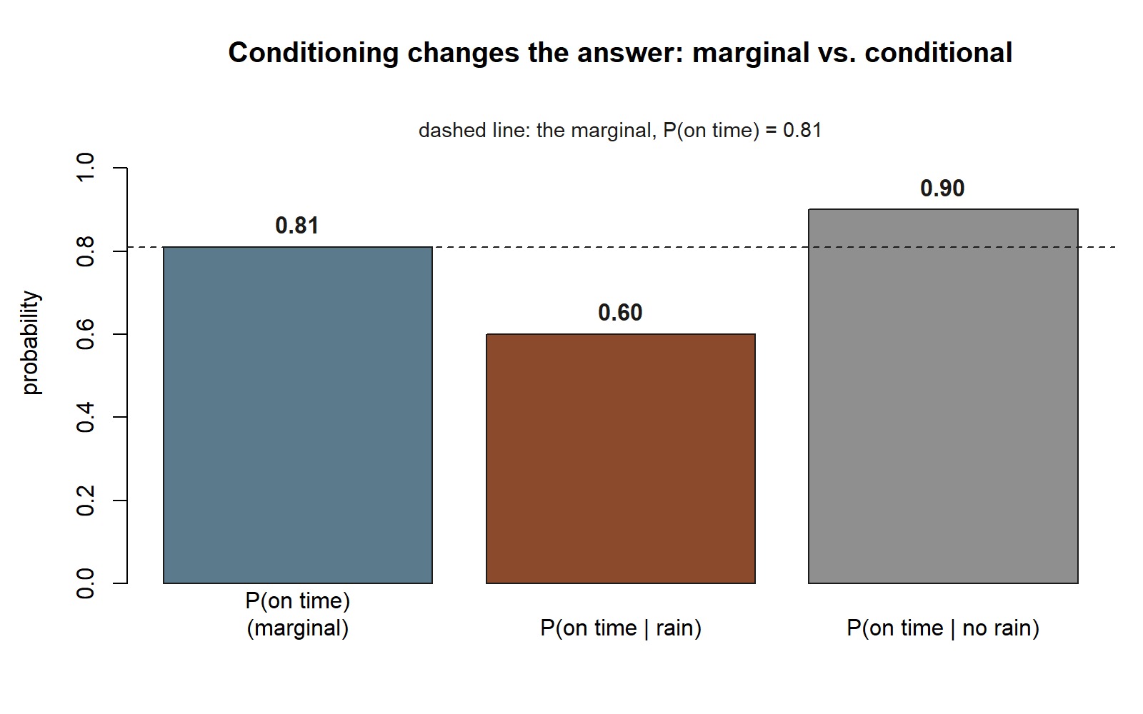
There is the term-long figure \(P(\text{on time}) = 0.81\). Now hold it next to the conditional \(P(T \mid R) = 0.60\). They are different numbers — and that difference is the whole point. The marginal \(0.81\) is what Maya should expect knowing nothing about today; the conditional \(0.60\) is what she should expect once she has looked out the window and seen rain. Knowing it is raining genuinely changes the answer, from \(0.81\) down to \(0.60\).

Figure 2: Marginal vs. conditional on-time rates (synthetic). The marginal \(P(\text{on time}) = 0.81\) sits between the two weather-conditional rates: rain pulls it down to \(0.60\), and no rain pushes it up to \(0.90\). The dashed line marks the marginal so the two conditional bars’ displacement from it is easy to read.

What the figure shows (non-visual equivalent). Three numbers on the same scale: the marginal \(0.81\), the rain-conditional \(0.60\) (below the marginal), and the no-rain-conditional \(0.90\) (above the marginal). Conditioning on the weather moves the on-time probability away from the marginal in the direction you would expect. Synthetic instructional example; numbers are illustrative.

Here is that same process drawn as a probability tree — the two-stage branching picture the multiplication rule builds, one branch per weather outcome and one sub-branch per on-time outcome:

Figure 3: The shuttle, as a probability tree (synthetic). Stage 1 branches on rain (0.30) vs. no rain (0.70); stage 2 branches on on time vs. late, with the conditional rate for the branch you are already on. Multiplying along a path gives that path’s probability; the four paths sum to \(1\).

What the figure shows (non-visual equivalent). Multiplying along each path: rain-then-on-time \(= 0.30 \times 0.60 = 0.18\); rain-then-late \(= 0.30 \times 0.40 = 0.12\); no-rain-then-on-time \(= 0.70 \times 0.90 = 0.63\); no-rain-then-late \(= 0.70 \times 0.10 = 0.07\). The four paths sum to \(1.00\), and the two on-time paths add to the marginal \(0.18 + 0.63 = 0.81\). Synthetic instructional example; numbers are illustrative.

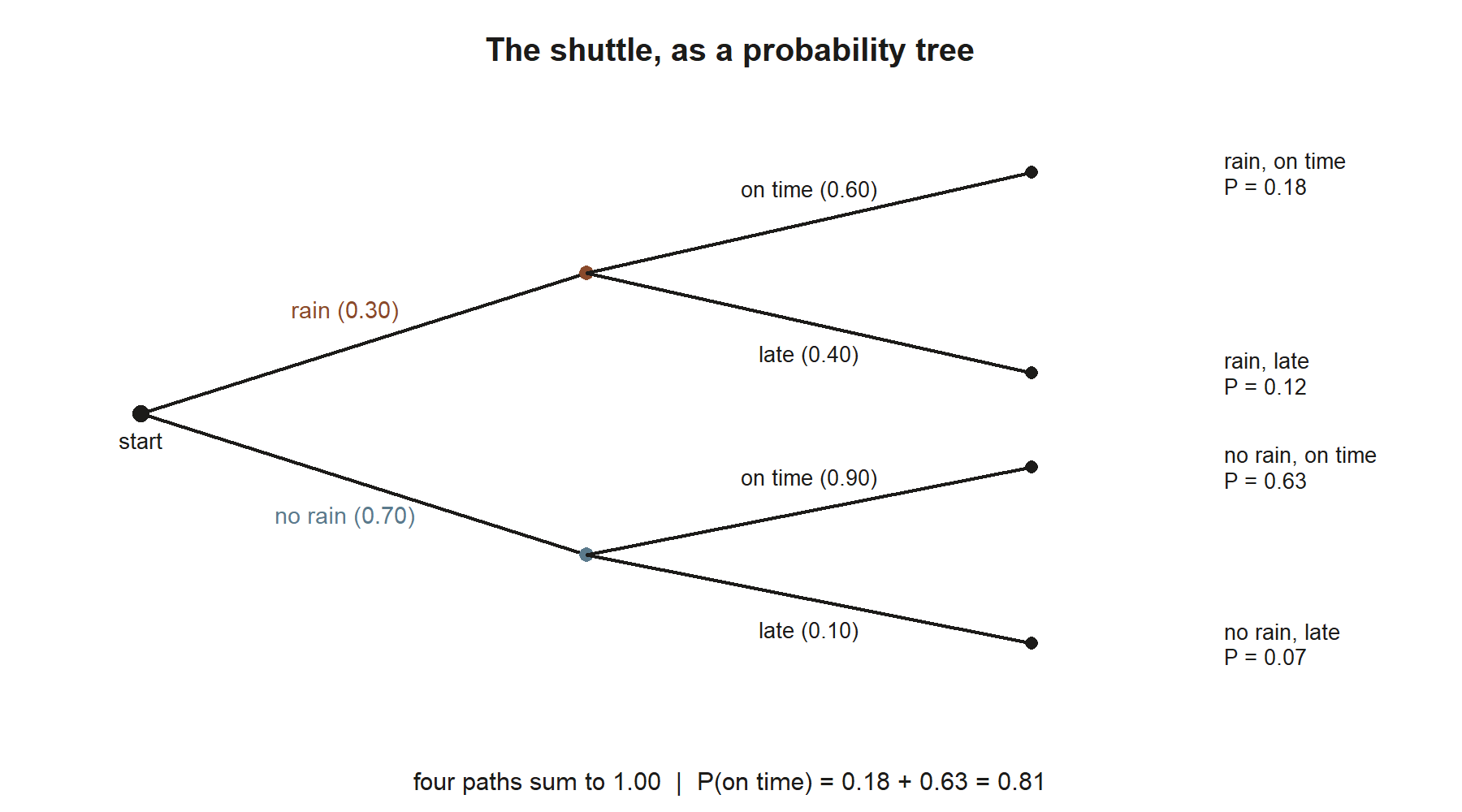
It is worth laying that same tree out as a small table — each row is one root-to-tip path, and the path probabilities sum to \(1\):

Table 1: Path-probability table: weather stage, on-time stage, and the multiplied path probability for each of the four root-to-tip paths; the numeric companion to the probability-tree figure above.

Weather (stage 1)	On time? (stage 2)	Path probability
Rain (\(0.30\))	On time (\(0.60\))	\(0.30 \times 0.60 = 0.18\)
Rain (\(0.30\))	Late (\(0.40\))	\(0.30 \times 0.40 = 0.12\)
No rain (\(0.70\))	On time (\(0.90\))	\(0.70 \times 0.90 = 0.63\)
No rain (\(0.70\))	Late (\(0.10\))	\(0.70 \times 0.10 = 0.07\)

The four paths total \(0.18 + 0.12 + 0.63 + 0.07 = 1.00\), as they must, and the two “on time” rows again give \(0.18 + 0.63 = 0.81\). We have just computed forward conditioning in full: the tree took us cleanly from the cause (weather) to the effect (on time). The reverse trip — from “late” back to “rain” — is the Week 5 story.

If you would like to see this as code (shown for teaching; not run in this build):

set.seed(35003)

p_rain      <- 0.30
p_ontime_R  <- 0.60   # P(on time | rain)
p_ontime_Rc <- 0.90   # P(on time | no rain)

# multiplication rule: joint path probabilities
joint_ontime_rain   <- p_ontime_R  * p_rain          # P(T and R)
joint_ontime_norain <- p_ontime_Rc * (1 - p_rain)    # P(T and R^c)

# marginal by adding the disjoint paths
p_ontime <- joint_ontime_rain + joint_ontime_norain  # 0.81

c(joint_ontime_rain = joint_ontime_rain,
  joint_ontime_norain = joint_ontime_norain,
  p_ontime = p_ontime)

Worked example — two cards, given the first is an ace (transfer)

Setup (symbolic). Take a standard, well-shuffled \(52\)-card deck and deal two cards without replacement — the first card is set aside, not returned, before the second is drawn. Let \(A_1\) be “the first card is an ace” and \(A_2\) be “the second card is an ace.” We want \(P(A_2 \mid A_1)\): given that the first card came up an ace, how likely is the second to be an ace too?

This is the same conditioning move in a brand-new setting. “Without replacement” is what makes the two draws depend on each other — what you see on the first draw changes the deck the second draw is taken from.

Reasoning it out (numeric). Condition on \(A_1\) by restricting to the world where the first card is an ace. In that world one ace is gone and one card removed: \(51\) cards remain, only \(3\) of them aces. The chance the next card is an ace is counted directly in the reduced deck:

\[ P(A_2 \mid A_1) = \frac{3}{51} = \frac{1}{17} \approx 0.0588. \]

Compare that to the unconditional chance that the second card is an ace, \(P(A_2) = 4/52 = 1/13 \approx 0.0769\). Conditioning on a first ace pulled the number down, because spending an ace on the first draw leaves fewer aces for the second. Once again, learning something changed the answer.

Figure 4: Two cards, without replacement, given the first is an ace (synthetic). The branch of the tree this example needs: given the first card is an ace (\(4/52\)), the second-draw branches become \(3/51\) (ace) and \(48/51\) (not ace). The other first-draw branch (first card not an ace) is shown but not expanded — it is not needed for \(P(A_2 \mid A_1)\).

What the figure shows (non-visual equivalent). Once you condition on the first card being an ace, the second draw is taken from a \(51\)-card deck holding only \(3\) aces, so \(P(A_2 \mid A_1) = 3/51 \approx 0.0588\) — lower than the unconditional \(P(A_2) = 4/52 \approx 0.0769\), because the first draw used up one of the four aces. The other first-draw branch (first card not an ace) is not needed for this question and is left unexpanded. Synthetic instructional example; numbers are illustrative.

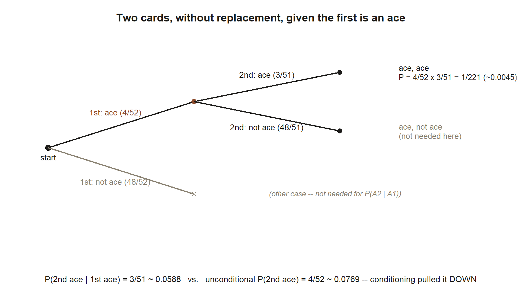
We can also confirm the definition gives the same value. Using \(P(A_1) = 4/52\) and the multiplication rule for the joint “both aces,”

\[ P(A_1 \cap A_2) = \frac{4}{52}\cdot\frac{3}{51} = \frac{12}{2652} = \frac{1}{221}, \]

\[ P(A_2 \mid A_1) = \frac{P(A_1 \cap A_2)}{P(A_1)} = \frac{1/221}{4/52} = \frac{3}{51} \approx 0.0588, \]

which matches the direct count. The definition and the “restrict the world” picture are two views of one idea.

A common mistake

The mistake that catches almost everyone first is reading the bar in the wrong direction — treating \(P(A \mid B)\) and \(P(B \mid A)\) as if they were the same number. They are emphatically not. In the shuttle world \(P(T \mid R) = 0.60\) is “given rain, on time,” while \(P(R \mid T)\) — “given the shuttle was on time, how likely is it that it rained” — is a different quantity entirely, and the reverse trip we are saving for Bayes. Whenever you write a conditional, say it out loud as “the probability of [left] given [right],” and make sure the thing on the right is genuinely the thing you are taking as known.

Figure 5: Two different directions (synthetic diagram). Left: the direction Week 3 actually computes — given rain (known), what is the chance of on time? Right: a different question the mistake confuses it with — given on time (known), what is the chance it rained? That reverse direction is not answered here; it needs Bayes’ rule, which waits until Week 5.

What the figure shows (non-visual equivalent). The two panels condition on different things. The left panel takes rain as known and asks about on-time — that is \(P(T \mid R) = 0.60\), the number this week computes. The right panel takes on-time as known and asks about rain — that is \(P(R \mid T)\), a different quantity this page does not compute; finding it needs Bayes’ rule (Week 5). Synthetic diagram; illustrative.

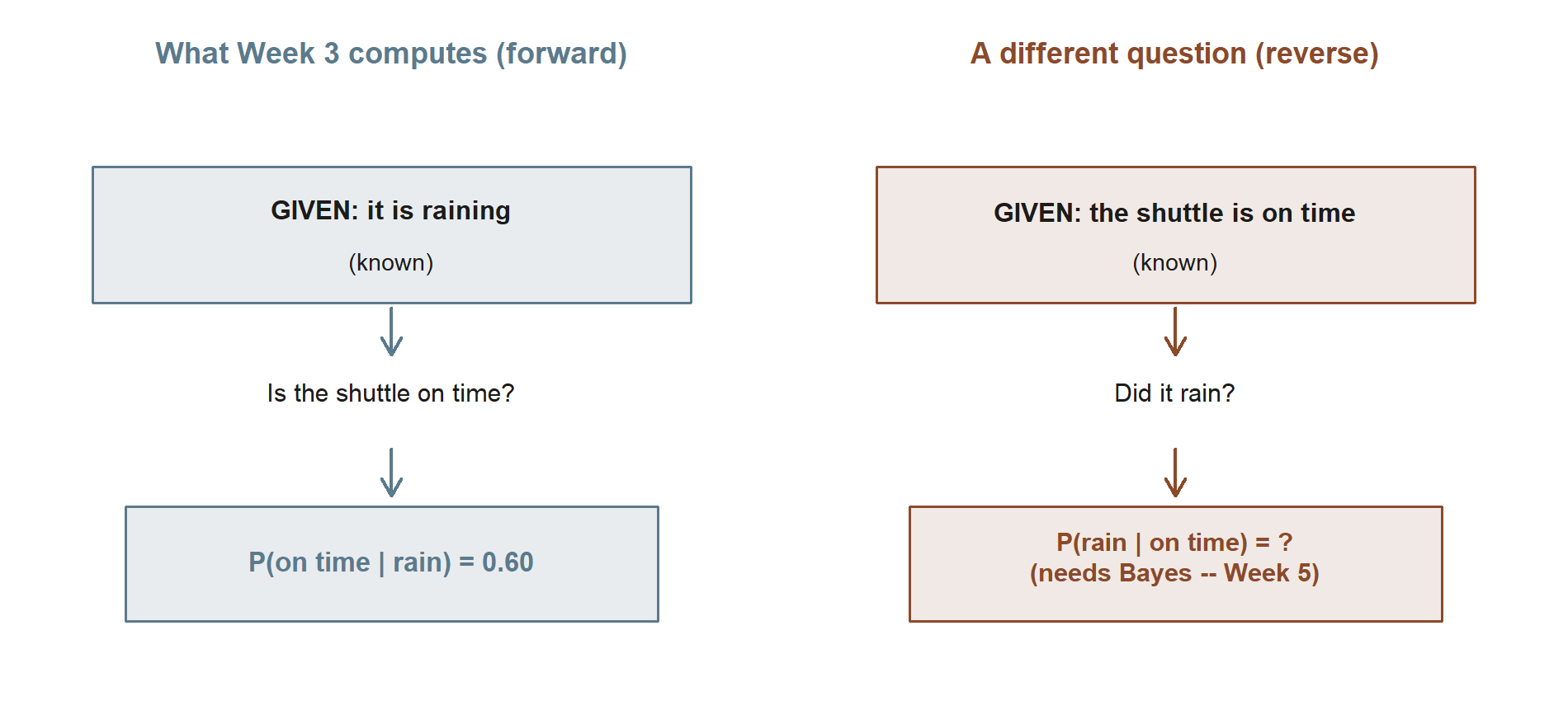
A close cousin of this slip is quoting the marginal when the conditional is what the situation calls for. If you already know it is raining, planning around \(P(T) = 0.81\) instead of \(P(T \mid R) = 0.60\) ignores the very information you have. And one precondition is easy to forget under pressure: \(P(A \mid B)\) only makes sense when \(P(B) > 0\). If \(B\) cannot happen, there is no world to condition on, and the expression is undefined rather than zero.

Low-stakes self-checks (ungraded)

Work these on your own; they are practice, not graded, and no answer key lives on this site.

1. In words, what is the difference between \(P(\text{on time} \mid \text{rain})\) and \(P(\text{on time})\)? Which one should Maya use on a morning when she has already seen rain, and why?
2. Using the shuttle numbers, find \(P(\text{late} \mid \text{rain})\) and \(P(\text{late} \mid \text{no rain})\) directly from the tree, then check that the four path probabilities still sum to \(1\).
3. Use the multiplication rule to write \(P(\text{rain and late})\) as a product of a conditional and a marginal, and compute it.
4. For the two-card example, redo the reasoning for \(P(\text{second card is an ace} \mid \text{first card is a king})\). Did conditioning change the second-draw chance this time? Explain why the answer differs from the first-ace case.
5. Explain, in one or two sentences, why \(P(A \mid B)\) requires \(P(B) > 0\). What would go wrong in the formula if \(P(B) = 0\)?

Reading and source pointer

For this week’s spine, read Grinstead & Snell, Introduction to Probability, Chapter 4 (Conditional Probability) — the definition of conditional probability, the multiplication rule, and the use of trees for staged experiments. The free online text is at https://www.dartmouth.edu/~chance/teaching_aids/books_articles/probability_book/book.html.

Alongside it, read the conditional-probability and independence material in MIT OpenCourseWare 18.05, Introduction to Probability and Statistics — its treatment of how a probability shifts once you condition, and its base-rate examples, set up nicely for the Bayes work in Week 5. The course is free at https://ocw.mit.edu/courses/18-05-introduction-to-probability-and-statistics-spring-2022/.

These notes are the course’s own synthesis, grounded in but not copied from the sources.

Public vs. graded

These notes, the examples, and the practice here are public and ungraded — study material only. No graded prompts, answer keys, rubrics, point values, or due dates appear on this site. Graded checkpoints, quizzes, homework, labs, the midterm, the project, and the final live in Blackboard (the LMS), which is authoritative for due dates, submissions, and grades. If this page and Blackboard ever disagree, follow Blackboard.

Looking ahead

Conditioning naturally raises its own follow-up question: when does conditioning change nothing at all? If learning \(B\) leaves \(P(A)\) exactly where it was, we call \(A\) and \(B\) independent — and Week 4 makes that precise, contrasting the shuttle (on-time and rain are not independent, since \(0.60 \neq 0.81\)) with a genuinely independent setup like successive coin tosses. Then Week 5 runs conditioning in reverse: the multiplication rule, written in both orders and combined with the law of total probability, becomes Bayes’ rule, which is how we get from “given rain, late” back to “given late, rain.” Everything we did with the forward tree this week is the scaffolding for that reversal.

See also

• Week 2 — Sample spaces, events & rules — the sample space, the complement, and the addition rule we lean on here.
• Week 4 — Independence & information — when conditioning leaves a probability unchanged.
• Week 5 — Bayes’ rule & updating — conditioning run in reverse.
• Notation glossary — the binding meaning of \(P(A \mid B)\), \(A \cap B\), and the rest of the symbols used above.
• Distribution reference — for the models that later get built by chaining conditional statements together.
• Course syllabus — the calendar (including the Labor Day no-class Monday) and the policies behind this week’s rhythm.