set.seed(35003)
# Synthetic joint pmf of X = rain (1/0) and Y = late (1/0); seed set.
# Cells: P(1,1)=0.12, P(1,0)=0.18, P(0,1)=0.07, P(0,0)=0.63.
n_mornings <- 200000
cells <- c("11", "10", "01", "00")
draws <- sample(cells, size = n_mornings, replace = TRUE,
                prob = c(0.12, 0.18, 0.07, 0.63))

x <- as.integer(substr(draws, 1, 1))   # rain indicator
y <- as.integer(substr(draws, 2, 2))   # late indicator

mean(x)                # estimates E[X]        -> near 0.30
mean(y)                # estimates E[Y]        -> near 0.19
mean(x * y)            # estimates E[XY]       -> near 0.12
cov(x, y)              # estimates Cov(X, Y)   -> near 0.063
cor(x, y)              # estimates rho         -> near 0.35
var(x + y)             # estimates Var(X + Y)  -> near 0.49

# Same numbers straight from the pmf, for comparison:
EX  <- 0.30; EY <- 0.19; EXY <- 0.12
EXY - EX * EY                                   # Cov = 0.063
(EXY - EX * EY) / sqrt(0.21 * 0.1539)           # rho ~ 0.35
0.21 + 0.1539 + 2 * (EXY - EX * EY) # Var(X + Y) = 0.4899Week 12 — Joint distributions & dependence
Marginal, conditional, covariance, correlation
Mathematical goal
Until now every random variable in this course has lived alone: one quiz count, one shuttle wait, one commute time. This week we let two random variables share the same experiment and ask how they move together. By the end you should be able to start from a joint probability mass function — a table of probabilities, one cell per pair of values — and produce, in order, every summary that describes the pair. Concretely, the week’s targets are:
- recovering each variable’s marginal pmf by summing the joint over the other variable, \(p_X(x)=\sum_y p(x,y)\) and \(p_Y(y)=\sum_x p(x,y)\);
- reading off a conditional pmf, \(p_{Y\mid X}(y\mid x)=p(x,y)/p_X(x)\) when \(p_X(x)>0\), and recognizing that this is just last term’s \(P(A\mid B)\) wearing random-variable clothing;
- computing the expectation of a product, \(E[XY]=\sum_x\sum_y xy\,p(x,y)\), and from it the covariance \(\operatorname{Cov}(X,Y)=E[XY]-E[X]E[Y]\), a signed measure of whether the two tend to move the same way;
- rescaling covariance into the unitless correlation \(\rho=\operatorname{Cov}(X,Y)/(\sigma_X\sigma_Y)\), which always lands in \([-1,1]\);
- and using the variance-of-a-sum rule \(\operatorname{Var}(X+Y)=\operatorname{Var}(X)+\operatorname{Var}(Y)+2\operatorname{Cov}(X,Y)\), the rule that finally explains why variances were allowed to simply add back in Week 8.
This is a derivation week, so the emphasis is on where each summary comes from and what it measures, not just on filling in a table. All worked numbers are synthetic (seed 35003 set) and held fixed.
The week question
We have spent the term building a running case around two events that have always seemed linked: whether it rains on a given morning, and whether Maya’s shuttle leaves her late. Back in Weeks 3–4 we found these were not independent — rain made lateness more likely — and in Week 5 we ran the link in reverse with Bayes’ rule. Up to now, though, “rain” and “late” were events. This week we promote them to random variables and ask the quantitative version of the same question:
Given the full joint distribution of two random variables \(X\) and \(Y\), how strongly, and in which direction, do they move together — and how do we boil that relationship down to a single number that does not depend on the units we happen to measure in?
The direction-and-strength question is answered by covariance; the units question is answered by correlation, which rescales covariance onto the fixed interval \([-1,1]\). We will derive both from the joint pmf and test them on the rain–late table, then carry the same machinery to a fresh height–weight example where the numbers are genuinely continuous in spirit.
Notation
| Symbol | Meaning |
|---|---|
| \(X,\,Y\) | two random variables sharing one experiment (capitals); values lowercase \(x,y\) |
| \(p(x,y)=P(X=x,\,Y=y)\) | joint pmf — probability of the pair \((x,y)\) occurring together |
| \(p_X(x)=\sum_y p(x,y)\) | marginal pmf of \(X\) — sum the joint over all \(y\) |
| \(p_Y(y)=\sum_x p(x,y)\) | marginal pmf of \(Y\) — sum the joint over all \(x\) |
| \(p_{Y\mid X}(y\mid x)=\dfrac{p(x,y)}{p_X(x)}\) | conditional pmf of \(Y\) given \(X=x\) (needs \(p_X(x)>0\)) |
| \(E[XY]=\sum_x\sum_y xy\,p(x,y)\) | expectation of the product of the two variables |
| \(\operatorname{Cov}(X,Y)=E[XY]-E[X]E[Y]\) | covariance — signed co-movement; same units as \(X\cdot Y\) |
| \(\rho=\dfrac{\operatorname{Cov}(X,Y)}{\sigma_X\,\sigma_Y}\) | correlation — covariance rescaled to \([-1,1]\), unitless |
| \(\sigma_X=\sqrt{\operatorname{Var}(X)}\) | standard deviation of \(X\) (and likewise \(\sigma_Y\)) |
| \(X\perp Y\) | \(X\) and \(Y\) independent: \(p(x,y)=p_X(x)\,p_Y(y)\) for every pair |
Two reminders carried in. First, a conditional only makes sense when you are conditioning on something with positive probability, exactly as in Week 3: \(p_{Y\mid X}(y\mid x)\) requires \(p_X(x)>0\). Second, covariance and correlation are not interchangeable — covariance carries the product of the two variables’ units and can be any real number, while correlation is unitless and bounded; this is convention-risk item 11 and we flag it again below.
Conceptual setup
A joint pmf is a probability table. When two discrete variables share an experiment, their full description is a single table \(p(x,y)\) assigning a probability to every pair of values, with all the cells non-negative and summing to \(1\). Everything else this week is extracted from that one table.
Marginals collapse the table. If you only care about \(X\), you no longer need the breakdown by \(Y\), so you add up each row (or column) of the joint:
\[ p_X(x) \;=\; \sum_y p(x,y), \qquad p_Y(y) \;=\; \sum_x p(x,y). \]
The word “marginal” is literal — historically these row-and-column totals were written in the margins of the table. Each marginal is itself a perfectly ordinary one-variable pmf, and Week 8’s \(E[X]\) and \(\operatorname{Var}(X)\) are computed from it exactly as before.
Conditionals re-weight one slice. Fixing \(X=x\) restricts attention to a single row of the table; dividing that row by its own total \(p_X(x)\) renormalizes it into a genuine pmf for \(Y\):
\[ p_{Y\mid X}(y\mid x) \;=\; \frac{p(x,y)}{p_X(x)}, \qquad p_X(x)>0. \]
This is identical to Week 3’s \(P(A\mid B)=P(A\cap B)/P(B)\), with the joint cell playing the role of the intersection and the marginal playing the role of \(P(B)\). Independence is the special case where conditioning changes nothing: \(X\perp Y\) exactly when \(p(x,y)=p_X(x)\,p_Y(y)\) for every pair, equivalently when \(p_{Y\mid X}(y\mid x)=p_Y(y)\).
Covariance measures co-movement. To ask whether \(X\) and \(Y\) tend to be large together, look at the product. Its expectation is taken against the joint pmf,
\[ E[XY] \;=\; \sum_x\sum_y xy\,p(x,y), \]
and then we subtract off what we would expect if the two were unrelated, \(E[X]E[Y]\), to define the covariance:
\[ \operatorname{Cov}(X,Y) \;=\; E\big[(X-\mu_X)(Y-\mu_Y)\big] \;=\; E[XY]-E[X]E[Y]. \]
The first form shows the meaning — average the product of the two deviations from their means — and the second is the computational shortcut, derived by expanding the product and using linearity exactly as we expanded \((X-\mu)^2\) for variance in Week 8. A positive covariance says above-average \(X\) tends to come with above-average \(Y\); a negative covariance says they tend to move oppositely; and zero covariance says there is no linear co-movement. Note that \(\operatorname{Cov}(X,X)=E[X^2]-(E[X])^2=\operatorname{Var}(X)\) — variance is just covariance of a variable with itself.
If \(X\perp Y\) then \(\operatorname{Cov}(X,Y)=0\). When the variables are independent, \(E[XY]=E[X]E[Y]\), so the covariance vanishes. The converse is not guaranteed — zero covariance means no linear relationship, not necessarily full independence — but for our purposes the headline is: dependence is exactly what makes covariance non-zero.
Correlation puts co-movement on a fixed scale. Covariance answers which direction, but its size is hostage to the units of \(X\) and \(Y\) — measure a height in centimetres instead of metres and the covariance inflates a hundredfold without the relationship changing at all. Dividing by both standard deviations cancels the units and the scale:
\[ \rho \;=\; \frac{\operatorname{Cov}(X,Y)}{\sigma_X\,\sigma_Y}, \qquad -1 \le \rho \le 1 . \]
The bound \(|\rho|\le 1\) is the Cauchy–Schwarz inequality in disguise; \(\rho=\pm 1\) exactly when \(Y\) is a perfect linear function of \(X\). Correlation keeps the sign of covariance but reports it as a pure strength-of-association number, comparable across any pair of variables.
Variances of a sum need the covariance term. Finally, combining two variables additively, the spread of the sum is
\[ \operatorname{Var}(X+Y) \;=\; \operatorname{Var}(X)+\operatorname{Var}(Y)+2\operatorname{Cov}(X,Y). \]
This is the missing piece from Week 8. There, the binomial variance \(np(1-p)\) came from adding up the variances of \(n\) indicator variables, and we promised it would be justified here: indicators of independent trials have zero covariance, so the cross term drops and the variances simply add. When the parts are not independent, the covariance term does not vanish, and the spread of the sum is inflated (positive covariance) or deflated (negative covariance) accordingly.
Worked example
We work the recurring rain–late pair symbolically first, then numerically, and watch each summary reconnect to a result we already trust from earlier weeks. Then a fresh transfer example — a small height–weight table — exercises the same machinery in a genuinely different context. Data are synthetic; seed 35003 set.
The recurring slice — rain and lateness as a joint distribution
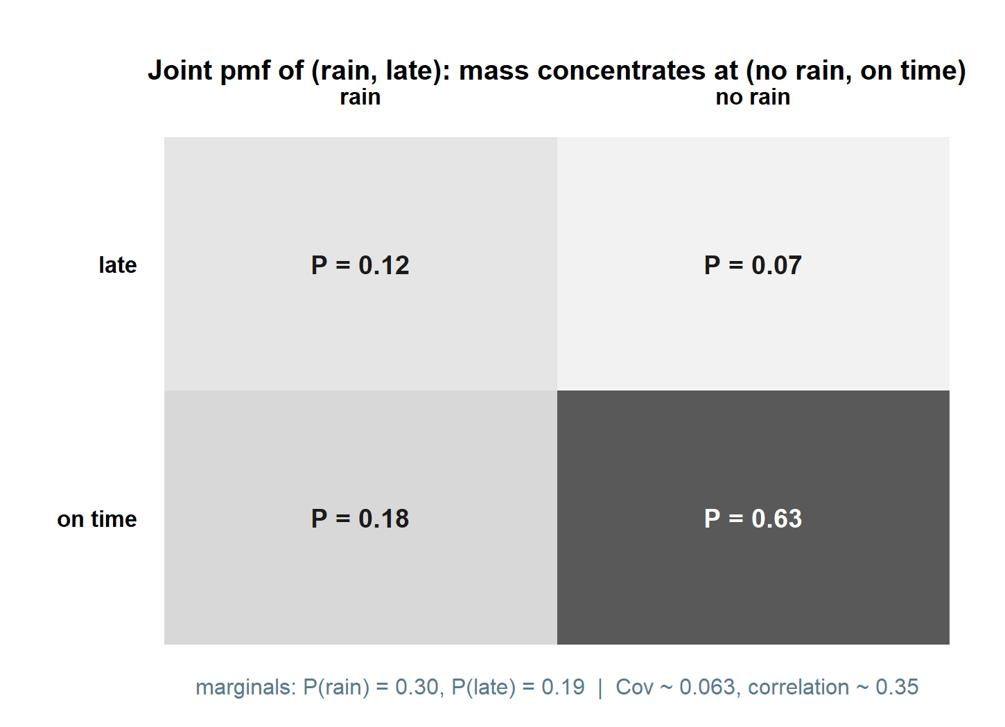
Let \(X=1\) if it rains on a given morning and \(X=0\) otherwise, and \(Y=1\) if Maya’s shuttle leaves her late and \(Y=0\) otherwise. From the running case we have the joint pmf
| \(Y=1\) (late) | \(Y=0\) (on time) | row total \(p_X(x)\) | |
|---|---|---|---|
| \(X=1\) (rain) | \(p(1,1)=0.12\) | \(p(1,0)=0.18\) | \(0.30\) |
| \(X=0\) (no rain) | \(p(0,1)=0.07\) | \(p(0,0)=0.63\) | \(0.70\) |
| col total \(p_Y(y)\) | \(0.19\) | \(0.81\) | \(1.00\) |
The four cells are non-negative and sum to \(0.12+0.18+0.07+0.63=1\), so this is a legitimate joint pmf.
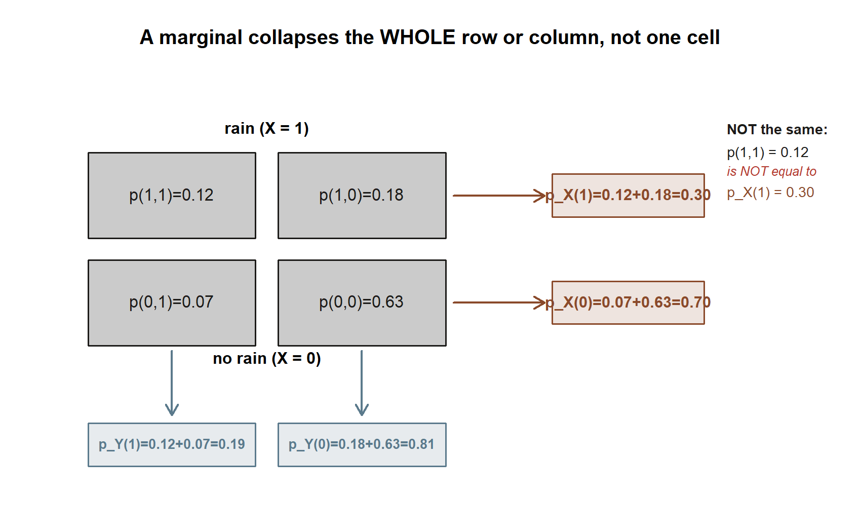
Marginals, by summing the table. Summing each row gives the rain marginal, and each column the lateness marginal:
\[ p_X(1)=0.12+0.18=0.30,\qquad p_X(0)=0.07+0.63=0.70, \] \[ p_Y(1)=0.12+0.07=0.19,\qquad p_Y(0)=0.18+0.63=0.81. \]
These are exactly the numbers we have carried all term: \(P(\text{rain})=0.30\) and \(P(\text{late})=0.19\). The joint table is internally consistent with the whole running case.
Conditionals, as a consistency check. Restrict to rainy mornings and renormalize:
\[ p_{Y\mid X}(1\mid 1)=\frac{p(1,1)}{p_X(1)}=\frac{0.12}{0.30}=0.40, \qquad p_{Y\mid X}(1\mid 0)=\frac{p(0,1)}{p_X(0)}=\frac{0.07}{0.70}=0.10. \]
So \(P(\text{late}\mid\text{rain})=0.40\) and \(P(\text{late}\mid\text{no rain})=0.10\) — these reproduce the Week 5 reverse-thread likelihoods exactly. The joint table is not a new world; it is the same commuter’s morning, repackaged so that two variables sit in one object. Because \(0.40\ne 0.10\), conditioning on rain genuinely changes the lateness distribution, which is the random-variable restatement of the Weeks 3–4 finding that on-time and rain are not independent.
Expectations, symbolically then numerically. Because \(X\) and \(Y\) are \(0/1\) indicators, their expectations are just the probabilities of the value \(1\):
\[ E[X]=1\cdot p_X(1)+0\cdot p_X(0)=p_X(1)=0.30, \qquad E[Y]=p_Y(1)=0.19. \]
The product \(XY\) equals \(1\) only on the single cell where both indicators are \(1\) — rain and late — so its expectation is just that one joint probability:
\[ E[XY]=\sum_{x}\sum_{y}xy\,p(x,y)=1\cdot1\cdot p(1,1)=0.12 . \]
(Every other term in the double sum has \(x=0\) or \(y=0\), so \(xy=0\).)
Covariance, from the computational formula.
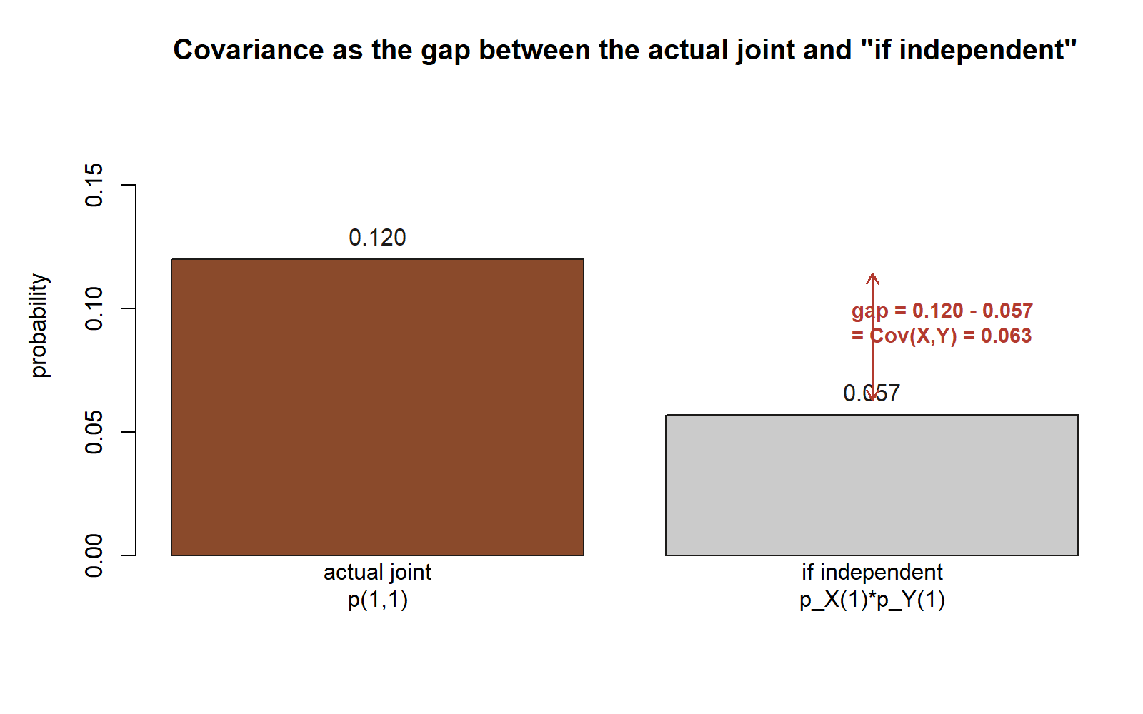
\[ \operatorname{Cov}(X,Y)=E[XY]-E[X]E[Y]=0.12-(0.30)(0.19)=0.12-0.057=0.063 . \]
The covariance is positive: rainy mornings go with late mornings, which is precisely the dependence we have been describing in words since Week 3, now expressed as a single signed number. If rain and lateness had been independent, we would have had \(E[XY]=E[X]E[Y]=0.057\) and a covariance of exactly \(0\); the gap of \(0.063\) between the joint \(0.12\) and the “if independent” \(0.057\) is the dependence.
Standard deviations of the two indicators. Each is a Bernoulli variable, whose variance is \(P(1)\cdot P(0)\):
\[ \operatorname{Var}(X)=(0.30)(0.70)=0.21, \qquad \operatorname{Var}(Y)=(0.19)(0.81)=0.1539, \]
so \(\sigma_X=\sqrt{0.21}\approx 0.4583\) and \(\sigma_Y=\sqrt{0.1539}\approx 0.3923\), giving \(\sigma_X\sigma_Y\approx 0.1798\).
Correlation, the unitless summary.
\[ \rho=\frac{\operatorname{Cov}(X,Y)}{\sigma_X\sigma_Y} =\frac{0.063}{\sqrt{0.21}\,\sqrt{0.1539}} =\frac{0.063}{0.1798} \approx 0.35 . \]
A correlation of about \(0.35\) is a moderate positive association: rain and lateness clearly move together, but the link is far from deterministic — plenty of rainy mornings are on time and plenty of dry mornings run late. The number sits comfortably inside \([-1,1]\), as every correlation must, and it carries no units, so it would be unchanged if we re-coded “late” as “minutes lost” on any scale.
Spread of the combined count. Suppose we form the simple total \(S=X+Y\), the number of “bad things” (rain, lateness) that happen on a morning, taking values \(0,1,2\). The variance-of-a-sum rule gives
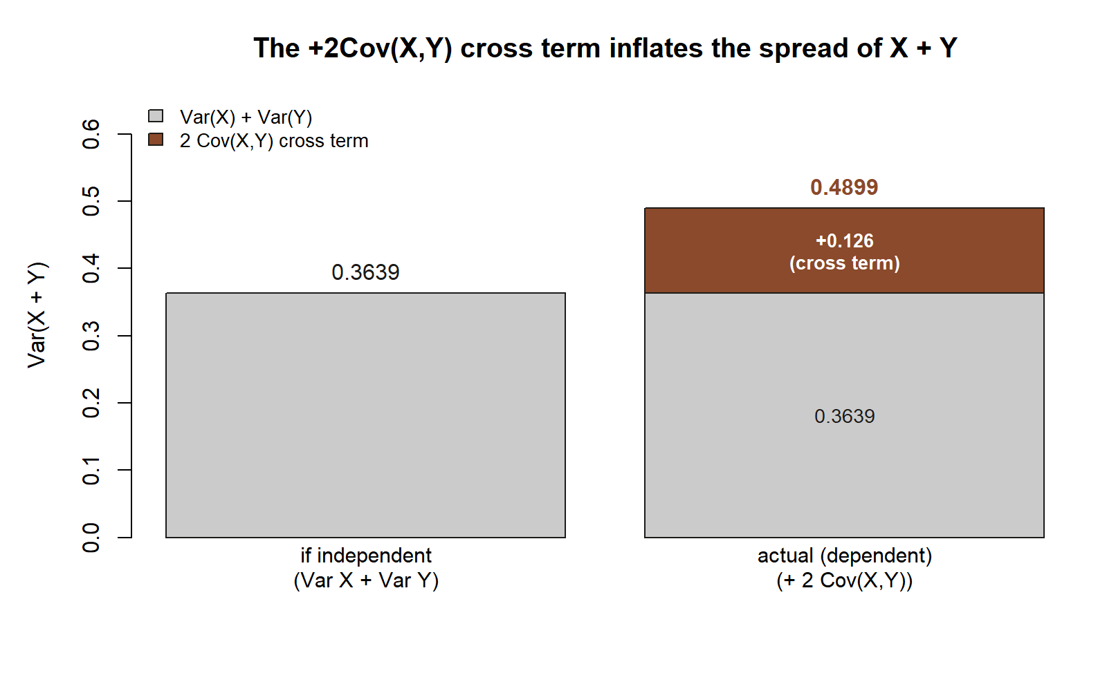
\[ \operatorname{Var}(X+Y)=\operatorname{Var}(X)+\operatorname{Var}(Y)+2\operatorname{Cov}(X,Y) =0.21+0.1539+2(0.063)=0.4899 . \]
Notice the cross term \(2(0.063)=0.126\) adds to the spread: because rain and lateness tend to arrive together, the combined count \(S\) swings a little wider than it would if the two were independent (where the variance would have been just \(0.21+0.1539=0.3639\)). That single line is the whole reason Week 8’s binomial variance was allowed to add variances — there the indicators were independent, the covariance was zero, and the cross term vanished.
You can see the same summaries by simulation; the chunk below is shown for teaching and is not run in this build. Run it in your own R session and the seed makes the result reproducible.
Transfer example — heights and weights move together
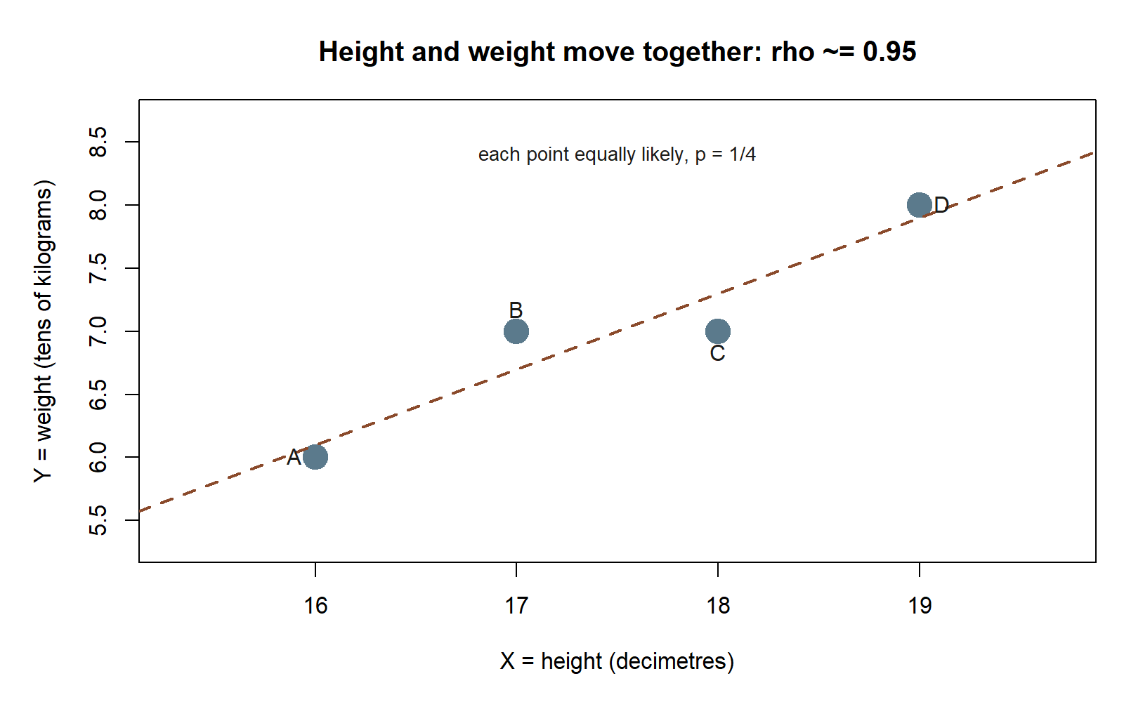
Now apply the same definitions in a brand-new context where both variables are quantitative rather than \(0/1\). Consider a tiny synthetic survey of four people, recorded as \(X=\) height (in decimetres, so \(16\) means \(160\) cm) and \(Y=\) weight (in tens of kilograms, so \(6\) means \(60\) kg), each pair equally likely with probability \(\tfrac14\). (Synthetic; seed 35003 set.)
| Person | \(X\) (height) | \(Y\) (weight) | \(p(x,y)\) |
|---|---|---|---|
| A | \(16\) | \(6\) | \(0.25\) |
| B | \(17\) | \(7\) | \(0.25\) |
| C | \(18\) | \(7\) | \(0.25\) |
| D | \(19\) | \(8\) | \(0.25\) |
Means.
\[ E[X]=\tfrac14(16+17+18+19)=\tfrac{70}{4}=17.5, \qquad E[Y]=\tfrac14(6+7+7+8)=\tfrac{28}{4}=7 . \]
Expectation of the product.
\[ E[XY]=\tfrac14\big(16\cdot6+17\cdot7+18\cdot7+19\cdot8\big) =\tfrac14\big(96+119+126+152\big)=\tfrac{493}{4}=123.25 . \]
Covariance.
\[ \operatorname{Cov}(X,Y)=E[XY]-E[X]E[Y]=123.25-(17.5)(7)=123.25-122.5=0.75 . \]
The covariance is positive — taller people tend to be heavier, as expected — but its value \(0.75\) is in the awkward unit “decimetres times ten-kilograms,” which means nothing on its own. So we rescale. The variances are
\[ E[X^2]=\tfrac14(16^2+17^2+18^2+19^2)=\tfrac14(256+289+324+361)=\tfrac{1230}{4}=307.5, \] \[ \operatorname{Var}(X)=307.5-(17.5)^2=307.5-306.25=1.25, \] \[ E[Y^2]=\tfrac14(36+49+49+64)=\tfrac{198}{4}=49.5, \qquad \operatorname{Var}(Y)=49.5-7^2=49.5-49=0.5 . \]
Correlation.
\[ \rho=\frac{\operatorname{Cov}(X,Y)}{\sigma_X\sigma_Y} =\frac{0.75}{\sqrt{1.25}\,\sqrt{0.5}} =\frac{0.75}{\sqrt{0.625}} =\frac{0.75}{0.7906} \approx 0.95 . \]
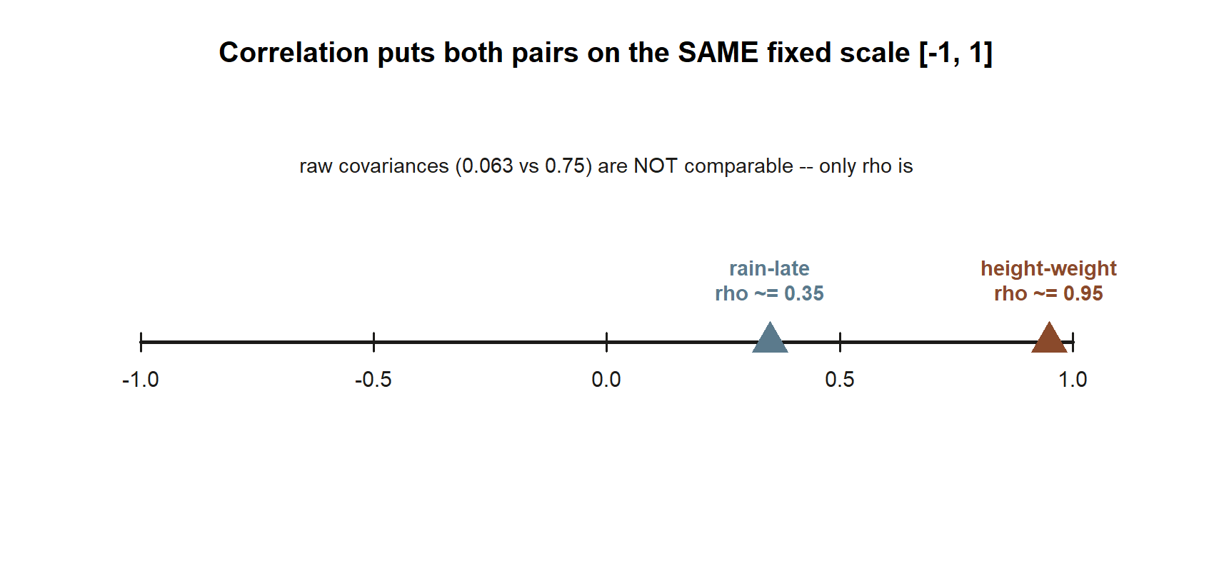
A correlation near \(0.95\) signals a very strong positive linear association — much tighter than the rain–late \(0.35\), which fits the picture: in this little table height and weight rise almost in lockstep, whereas rain only nudges lateness. The same two formulas, applied to a completely different pair of variables, again land a unitless number safely inside \([-1,1]\) — and crucially, that number is unchanged if we had kept height in centimetres and weight in kilograms, because correlation is blind to units.
A convention warning
A few places where the algebra of two variables quietly bites, several of them on this week’s convention-risk list:
- Covariance is unbounded; correlation lives in \([-1,1]\) (convention-risk item 11). Covariance carries the product of the two variables’ units and can be any real number, so its raw size tells you little — the rain–late covariance \(0.063\) and the height–weight covariance \(0.75\) are not comparable. Only after dividing by \(\sigma_X\sigma_Y\) to get \(\rho\) (\(0.35\) versus \(0.95\)) can you compare strengths across pairs. Always rescale before you interpret magnitude.
- A marginal is a sum, not a single cell. \(p_X(1)=0.30\) is \(p(1,1)+p(1,0)=0.12+0.18\), not the rainy-and-late cell \(0.12\) alone. Reading a corner cell as a marginal is a common slip; the marginal always collapses the whole row or column.
- The variance of a sum is not just the sum of variances. \(\operatorname{Var}(X+Y)\) carries the extra term \(2\operatorname{Cov}(X,Y)\). Dropping it is only legal when the covariance is zero — for instance when \(X\perp Y\). For the dependent rain–late pair the cross term contributes \(0.126\) of the total \(0.4899\); ignoring it understates the spread.
- Independence forces zero covariance, but the reverse is not guaranteed. \(X\perp Y\Rightarrow \operatorname{Cov}(X,Y)=0\), yet \(\operatorname{Cov}(X,Y)=0\) does not by itself prove independence — covariance only sees linear co-movement, and a variable can depend on another in a curved way that averages out to zero covariance. Treat “zero covariance” as “no linear association,” not as “independent.”
- A conditional needs a positive-probability condition. \(p_{Y\mid X}(y\mid x)=p(x,y)/p_X(x)\) is defined only when \(p_X(x)>0\), exactly the Week 3 precondition \(P(B)>0\). Never divide a joint cell by a zero marginal.
Practice (ungraded)
Work these for yourself; they are ungraded self-checks, not submissions. Each should fall straight out of this week’s definitions and rules — no new machinery needed.
- From the rain–late joint table, recompute both marginals by summing rows and columns, and confirm \(p_X(1)=0.30\) and \(p_Y(1)=0.19\). Then verify the four cells add to \(1\).
- Compute the two conditionals \(P(\text{late}\mid\text{rain})\) and \(P(\text{late}\mid\text{no rain})\) from the table, and check they equal \(0.40\) and \(0.10\) — the Week 5 reverse-thread likelihoods.
- Reproduce \(E[XY]=0.12\), then \(\operatorname{Cov}(X,Y)=0.063\), then \(\rho=0.063/(\sqrt{0.21}\sqrt{0.1539})\approx 0.35\), showing each step. Confirm \(\rho\) lies in \([-1,1]\).
- Using the variance-of-a-sum rule, compute \(\operatorname{Var}(X+Y)\) for the rain–late pair, then redo it as if \(X\) and \(Y\) were independent (drop the covariance term) and explain in one sentence why the dependent answer is larger.
- For the height–weight table, re-derive \(\operatorname{Cov}(X,Y)=0.75\) and \(\rho\approx 0.95\) from the definitions. Then argue in one or two sentences why \(\rho\) would be unchanged if height were recorded in centimetres and weight in kilograms, even though the covariance would change.
Reading and source pointer
For this week, read Grinstead & Snell, Introduction to Probability, Chapter 6 — Expected Value and Variance (for \(E[XY]\) and the covariance/variance algebra) and Chapter 7 — Sums of Random Variables (for how two variables combine and how their spread adds), in the free online text: https://www.dartmouth.edu/~chance/teaching_aids/books_articles/probability_book/book.html. Those chapters develop expectation of a product, covariance, and the variance of a sum — the same scaffold this note builds, in the same order. (No MIT 18.05 pointer is assigned this week; it returns in Week 13 with the simulation/limit-behavior strand.)
These notes are the course’s own synthesis, grounded in but not copied from the sources. All examples and numbers here are original and synthetic (seed 35003 set); none are taken from the text’s examples, exercises, figures, or solutions.
Public vs. graded
These notes, the examples, and the practice here are public and ungraded — study material only. No graded prompts, answer keys, rubrics, point values, or due dates appear on this site. Graded checkpoints, quizzes, homework, labs, the midterm, the project, and the final live in Blackboard (the LMS), which is authoritative for due dates, submissions, and grades. If this page and Blackboard ever disagree, follow Blackboard.
Looking ahead
You can now describe how two random variables move together — marginals, conditionals, covariance, correlation, and the variance of their sum. The variance-of-a-sum rule in particular is the hinge into next week: when many variables are added (or averaged), their covariances control how the spread of the total behaves. Next week we let \(n\) grow and watch what happens to the average of many independent commute times — the law of large numbers (the average settles onto \(E[X]\)) and the central limit theorem (the average’s distribution becomes approximately normal). The cross-term you met here is exactly why independence makes those limit results so clean, and Week 13 reaches them by simulation.
See also
- Week 3 — Conditional probability — where \(P(\text{late}\mid\text{rain})\) and the rain–lateness dependence first appeared; this week reproduces those conditionals from the joint pmf.
- Week 5 — Bayes’ rule & updating — the reverse-thread likelihoods \(0.40\) and \(0.10\) that the joint table reproduces exactly.
- Week 8 — Expectation & variance — the \(E[X]\), \(\operatorname{Var}(X)\), and “variances add” promise that the covariance term here finally justifies.
- Week 13 — Sums, simulation & limit behavior — where the variance-of-a-sum rule grows into the law of large numbers and the central limit theorem.
- Notation glossary — the binding symbols for \(\operatorname{Cov}(X,Y)\), \(\rho\in[-1,1]\), joint and marginal pmfs.
- Distribution reference — quick mean/variance facts for the standard models, with parameterizations fixed.
- Course syllabus — schedule, policies, and where graded work lives.