set.seed(35003)
n_quizzes <- 100000
# each quiz: 10 true/false questions, guessed; count the correct ones
correct <- replicate(n_quizzes, sum(sample(c(0, 1), size = 10, replace = TRUE)))
empirical <- table(factor(correct, levels = 0:10)) / n_quizzes
theoretical <- choose(10, 0:10) / 2^10
round(rbind(empirical, theoretical), 3) # the two rows should nearly matchWeek 7 — Discrete random variables
Turning outcomes into numbers: random variables and pmfs
The week question
Last week you learned to count outcomes: how many ways the chips can land, how many ways a hand can be dealt, how many ways to get exactly \(k\) correct on a quiz. Counting tells you how many outcomes there are and how likely each one is, but it leaves the answer scattered across a list of possibilities. This week we ask a tidier question.
When the thing we actually care about is a number — a count, a total, a score — how do we package the whole probability picture for that number in one place?
The answer is the random variable. A random variable does one simple, powerful thing: it attaches a number to each outcome of an experiment. Once outcomes become numbers, we can line them up on a number line, ask “what is the probability the number equals 3?”, and collect every such answer into a single object called a probability mass function. By the end of the week you should be able to take a chance experiment, define a random variable for it, write down its pmf, and read off probabilities of the form “exactly this many” and “this many or fewer.”
Why this matters
Almost every probability question a person actually asks in the wild is about a number: how many shuttles will be late this week, how many of the ten quiz questions you will get right, how many heads in a handful of coin flips, how long until the next bus. The random variable is the bridge between the messy list of outcomes you built in Weeks 1 through 6 and the numeric questions that come next.
It also sets up everything that follows. Once a number has a probability distribution, you can ask for its average (Week 8, expectation) and its spread (Week 8, variance). You can notice that many different experiments share the same distribution and give it a name (Week 9, the binomial and Poisson; Weeks 10–11, the continuous models). The pmf you meet this week is the discrete ancestor of the density curve you will meet for continuous quantities. Getting comfortable now with “outcome in, number out, probability attached” makes the rest of the course feel like variations on one idea rather than a parade of new ones.
This week also sits at a natural checkpoint. We have finished building the discrete-probability toolkit, so it is a good moment to consolidate before the course turns toward averages, named models, and continuous quantities. See Looking ahead for how that checkpoint frames your studying.
Learning goals
By the end of this week you should be able to:
- Define a discrete random variable as a rule that assigns a number to each outcome of an experiment.
- Write the probability mass function \(p(x)=P(X=x)\) for a simple experiment and check that it is a valid pmf (each value in \([0,1]\), and all values summing to \(1\)).
- Build and read the cumulative distribution function \(F(x)=P(X\le x)\) from a pmf.
- Translate a plain-language question (“at least 8 correct”, “fewer than 2 heads”) into a statement about \(X\) and evaluate it from the pmf or cdf.
- Distinguish a random variable \(X\) (the rule / the capital letter) from a particular value \(x\) (a number it can take), and read \(p(x)\) and \(P(X=x)\) as two names for the same thing.
Core vocabulary
- Random variable \(X\) — a rule that assigns a real number to every outcome \(\omega\) in the sample space \(\Omega\). We write random variables with capital letters; the values they take are lowercase \(x\).
- Discrete random variable — a random variable whose possible values form a list you can write out (finite, like \(0,1,\dots,10\), or a countable sequence). This week is entirely about the discrete kind.
- Support — the set of values \(x\) for which \(p(x)>0\); the numbers \(X\) can actually take.
- Probability mass function (pmf) \(p(x)=P(X=x)\) — the function that reports the probability that \(X\) equals each value \(x\). Sometimes written \(p_X(x)\) when we need to say which variable. A valid pmf has \(0\le p(x)\le 1\) for every \(x\) and \(\sum_x p(x)=1\).
- Cumulative distribution function (cdf) \(F(x)=P(X\le x)\) — the running total of the pmf: the probability that \(X\) is at most \(x\). It climbs from \(0\) up to \(1\) as \(x\) moves left to right.
- Distribution — the whole package: the support together with the probabilities attached to it. The pmf (or the cdf) is the distribution of a discrete random variable.
Concept development
From outcomes to numbers
Up to now an outcome has been a thing — a “heads,” a “rain-then-late morning,” a particular pattern of right and wrong quiz answers. A random variable is the small, deliberate act of replacing each such thing with a number we care about.
Formally, a random variable \(X\) is a function from the sample space to the real numbers: feed it an outcome \(\omega\), and it returns a number \(X(\omega)\). That sounds abstract, but the move is one you make instinctively. Flip three coins and you might not care about the exact pattern HTH versus THH; you care that two heads came up. The phrase “number of heads” is a random variable: it takes each three-flip outcome and returns \(0\), \(1\), \(2\), or \(3\).
The point of the function is that it lets several different outcomes collapse onto the same number. Both HTH and THH and HHT return the value \(2\). That is exactly what we want: the number of heads does not care which particular pattern produced it. The probabilities of those outcomes then pile up on the value \(2\), and that pile is what the pmf records.
The probability mass function
Once \(X\) turns outcomes into numbers, we can ask a clean question for each possible value: what is the probability that \(X\) equals this number? The function that answers it for every value at once is the probability mass function,
\[ p(x) = P(X = x). \]
Read it as “the probability mass sitting at the value \(x\).” For a discrete variable, all of the probability in the experiment gets distributed — as discrete lumps — onto the values in the support. To find \(p(x)\) you gather every outcome that \(X\) sends to \(x\) and add up their probabilities:
\[ p(x) = P(X = x) = \sum_{\omega : X(\omega) = x} P(\{\omega\}). \]
Two conditions make a function a legitimate pmf, and they are worth checking every time you write one down. First, no value can carry negative or impossible probability:
\[ 0 \le p(x) \le 1 \quad \text{for every } x. \]
Second, the masses must account for all of the probability — the experiment certainly produces some value — so they sum to one over the support:
\[ \sum_{x} p(x) = 1. \]
If a pmf you have written fails the sum-to-one check, you have either missed a value or mis-counted one; the check is your first line of defense against an arithmetic slip.
A small but important notation note from the course ledger: for a discrete random variable, \(p(x)\) and \(P(X=x)\) are simply two names for the same number. We use \(p(x)\) when we want to emphasize the function (the whole table of probabilities) and \(P(X=x)\) when we want to emphasize a single probability we are computing. Do not let the two notations make you think they are different objects.
The cumulative distribution function
The pmf answers “exactly this value.” Many real questions instead ask “this value or fewer”: at most two late shuttles, fewer than five correct, no more than one defect. For these we accumulate the pmf from the bottom up. The cumulative distribution function is
\[ F(x) = P(X \le x) = \sum_{t \le x} p(t), \]
the total probability mass at or below \(x\). Because we are piling up non-negative lumps as \(x\) increases, \(F\) has three features that hold for every discrete random variable:
- It starts at \(0\) (below the smallest value, no mass has accumulated) and ends at \(1\) (above the largest value, all the mass is in).
- It never decreases as \(x\) moves right — adding more lumps can only keep the total the same or raise it.
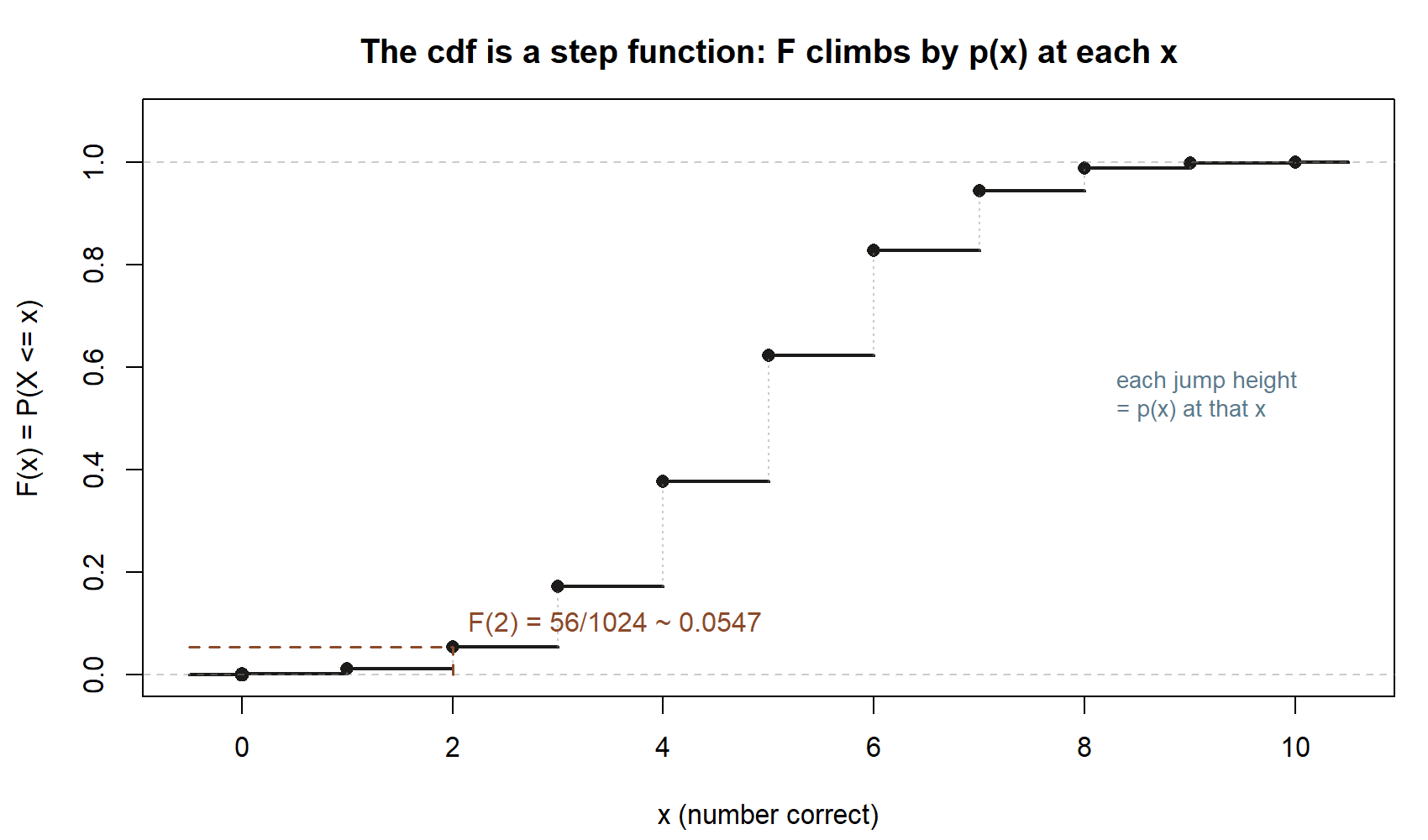
- For a discrete variable it is a step function: flat between the support values, jumping up by exactly \(p(x)\) at each value \(x\). The size of each jump is the pmf at that point, which means you can recover the pmf from the cdf and vice versa.
The cdf earns its keep on “tail” questions. The probability of “more than \(a\)” is the complement of “at most \(a\)”:
\[ P(X > a) = 1 - F(a), \]
and the probability of landing in a block of values is a difference of cdf values,
\[ P(a < X \le b) = F(b) - F(a). \]
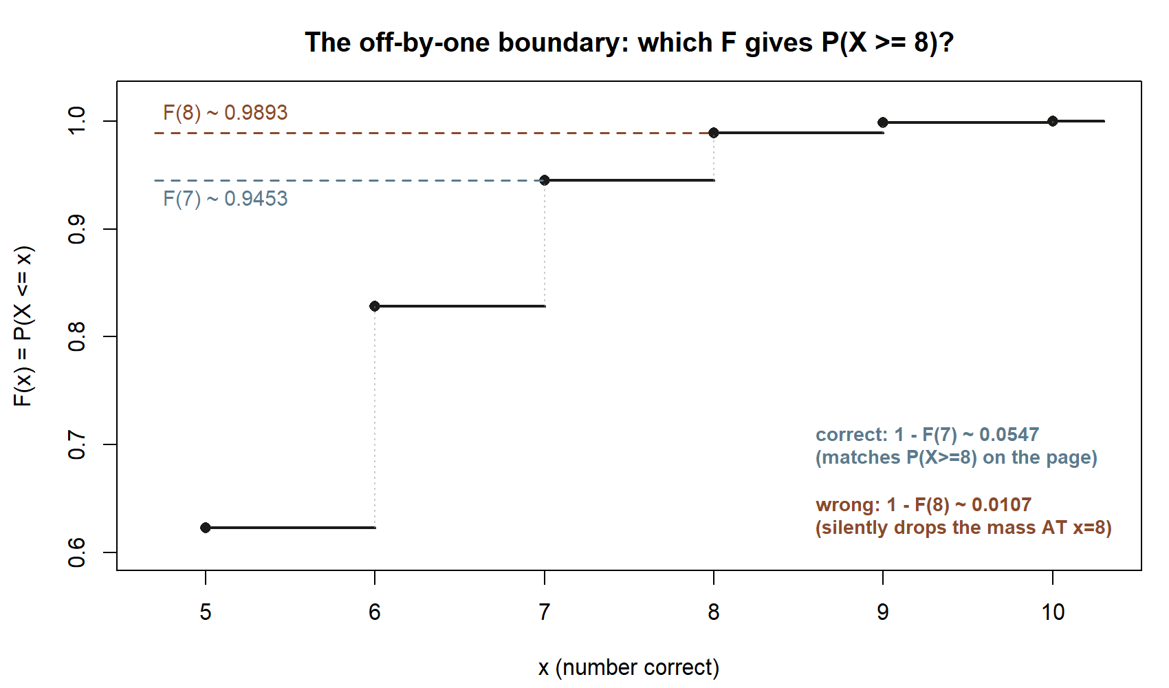
Be careful with the boundary: \(P(X \ge a)\) for an integer-valued variable is \(1 - F(a-1)\), not \(1-F(a)\), because \(F(a)\) already includes the mass at \(a\). That one-step boundary care is the most common place a correct pmf still yields a wrong tail probability.
Worked examples
Each example moves from the symbolic pmf to specific numbers. The data are synthetic; seed 35003 is set for any simulation a student might run.
Worked example — the quiz, as a random variable (recurring case)
Throughout the course we follow Maya, a commuter student. Last week we counted her ten-question true/false quiz: with pure guessing, each question is right with probability \(0.5\), the \(2^{10}=1024\) answer keys are equally likely, and the number of keys giving exactly \(k\) correct answers is \(\binom{10}{k}\). This week we name the quantity she actually cares about and package it.
Define the random variable. Let
\[ X = \text{the number of the ten questions Maya gets correct by guessing.} \]
Each outcome of the experiment is one full answer key (one of the \(1024\) equally likely right/wrong patterns); \(X\) sends each key to its count of correct answers. The support is \(0,1,2,\dots,10\).
Build the pmf symbolically. All \(1024\) keys are equally likely, and \(\binom{10}{x}\) of them have exactly \(x\) correct. So the probability mass at \(x\) is the fraction of keys that hit \(x\):
\[ p(x) = P(X = x) = \frac{\binom{10}{x}}{2^{10}} = \binom{10}{x}\left(\tfrac{1}{2}\right)^{10}, \qquad x = 0,1,2,\dots,10. \]
(You will meet this exact shape again in Week 9 under its proper name, the binomial pmf. For now it is just “equally likely keys, counted.”)
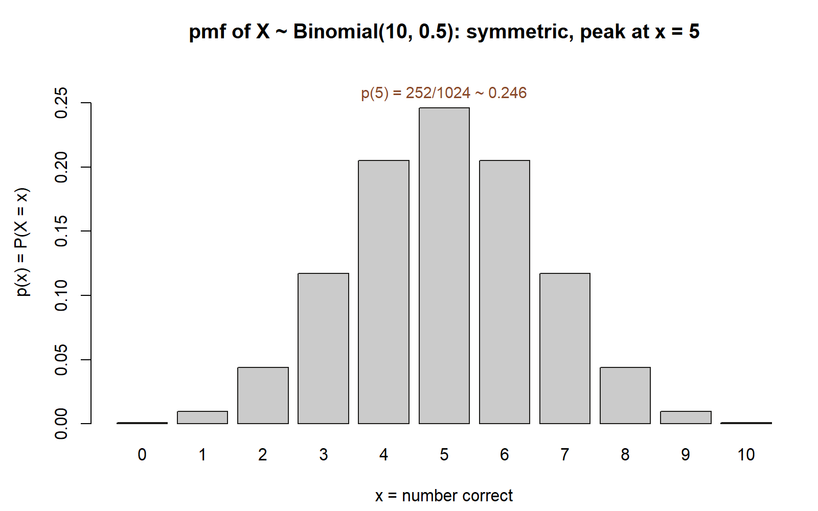
Put numbers on it. Since \((1/2)^{10} = 1/1024\), the pmf is each binomial coefficient over \(1024\). The coefficients across the row are \(1,10,45,120,210,252,210,120,45,10,1\) — symmetric, because guessing has no bias toward right or wrong. Reading off a few values:
| \(x\) | \(\binom{10}{x}\) | \(p(x)=P(X=x)\) |
|---|---|---|
| 0 | 1 | \(1/1024\approx 0.001\) |
| 1 | 10 | \(10/1024\approx 0.010\) |
| 2 | 45 | \(45/1024\approx 0.044\) |
| 5 | 252 | \(252/1024\approx 0.246\) |
| 8 | 45 | \(45/1024\approx 0.044\) |
| 9 | 10 | \(10/1024\approx 0.010\) |
| 10 | 1 | \(1/1024\approx 0.001\) |
The masses are largest in the middle, around \(x=5\) — which already hints that pure guessing tends to land near half-right, the average we will pin down precisely in Week 8.
Check the pmf. Every value is between \(0\) and \(1\), and the coefficients sum to \(1+10+45+120+210+252+ 210+120+45+10+1 = 1024\), so
\[ \sum_{x=0}^{10} p(x) = \frac{1024}{1024} = 1. \checkmark \]
Read the cdf for a tail question. Suppose Maya wants the probability she scores at most \(2\) correct. That is a cdf value:
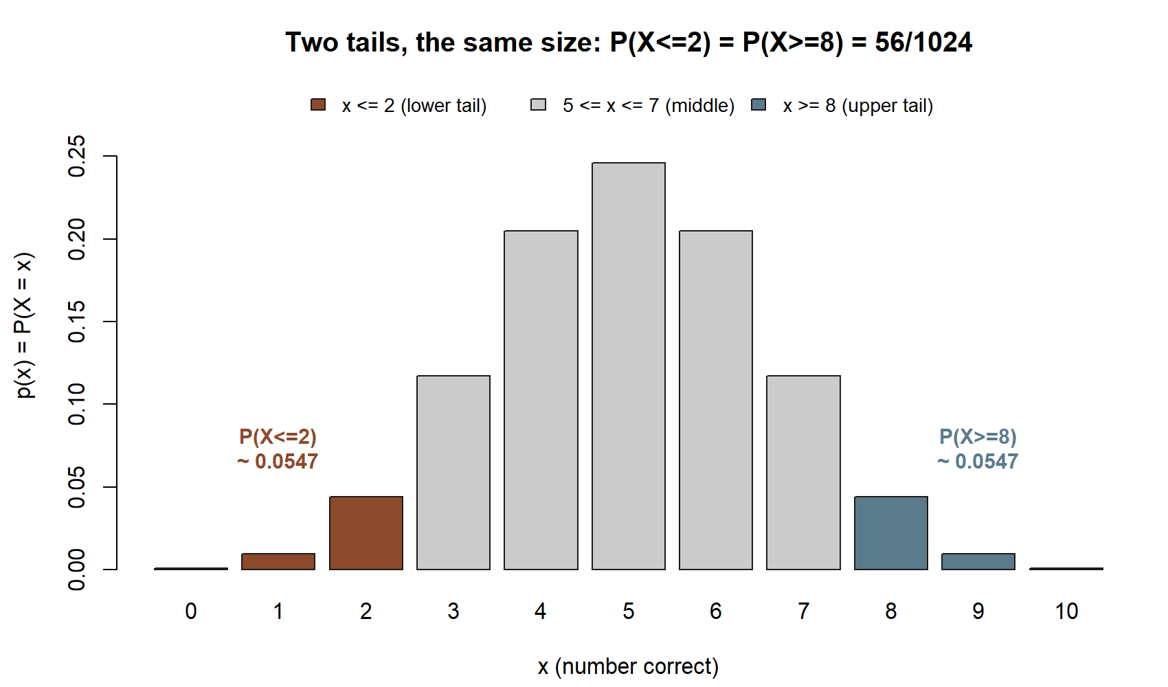
\[ F(2) = P(X \le 2) = p(0)+p(1)+p(2) = \frac{1+10+45}{1024} = \frac{56}{1024} \approx 0.0547. \]
And the complementary “she gets at least \(8\) correct” question reads off the symmetric upper tail:
\[ P(X \ge 8) = p(8)+p(9)+p(10) = \frac{45+10+1}{1024} = \frac{56}{1024} \approx 0.0547, \]
equal to the lower tail because the distribution is symmetric. (We revisit exactly this \(P(X\ge 8)\approx 0.0547\) in Week 9 once the variable wears its binomial name.) Notice the boundary care from the concept section: “\(X\ge 8\)” is \(1-F(7)\), not \(1-F(8)\).
So the move this week is not new probability — it is repackaging. The counting you did in Week 6 is the pmf; the random variable just gives the count a name and a number line to live on.
Worked example — number of heads in three coin flips (transfer)
Now carry the same machinery to a fresh, smaller experiment so the pattern stands on its own. Flip a fair coin three times and let
\[ X = \text{the number of heads in three flips.} \]
Symbolic setup. The sample space is the eight equally likely flip patterns, \(\{\text{HHH}, \text{HHT}, \text{HTH}, \text{THH}, \text{HTT}, \text{THT}, \text{TTH}, \text{TTT}\}\), each of probability \(1/8\). The random variable \(X\) counts the heads in each pattern, so its support is \(\{0,1,2,3\}\). The mass at \(x\) is the number of patterns with exactly \(x\) heads, divided by \(8\):
\[ p(x) = P(X = x) = \frac{\binom{3}{x}}{2^{3}} = \frac{\binom{3}{x}}{8}, \qquad x = 0,1,2,3. \]
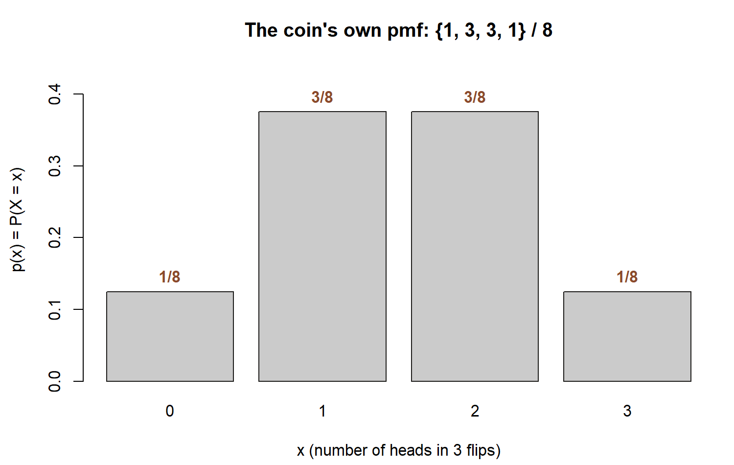
Numeric pmf. The coefficients \(\binom{3}{0},\binom{3}{1},\binom{3}{2},\binom{3}{3}\) are \(1,3,3,1\), so the pmf is the tidy table
| \(x\) | patterns | \(p(x)\) |
|---|---|---|
| 0 | TTT | \(1/8 = 0.125\) |
| 1 | HTT, THT, TTH | \(3/8 = 0.375\) |
| 2 | HHT, HTH, THH | \(3/8 = 0.375\) |
| 3 | HHH | \(1/8 = 0.125\) |
— the famous \(\{1,3,3,1\}/8\). It passes both validity checks: every entry lies in \([0,1]\), and \(\tfrac{1}{8}+\tfrac{3}{8}+\tfrac{3}{8}+\tfrac{1}{8}=\tfrac{8}{8}=1\).
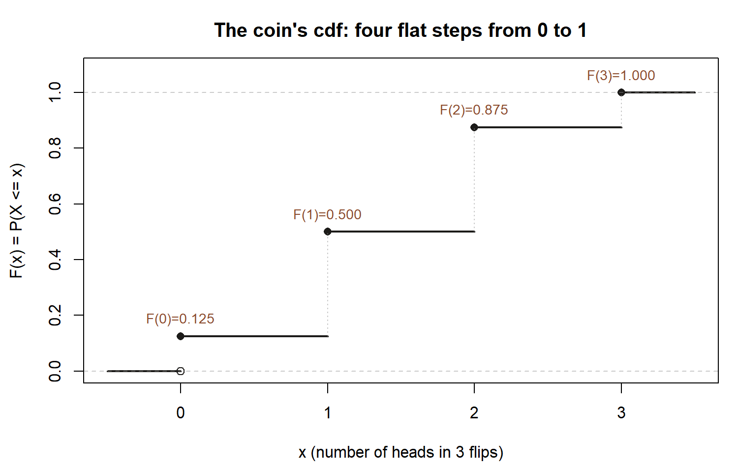
Build the cdf. Accumulate the pmf from the left:
\[ F(0)=\tfrac{1}{8}=0.125,\quad F(1)=\tfrac{4}{8}=0.5,\quad F(2)=\tfrac{7}{8}=0.875,\quad F(3)=\tfrac{8}{8}=1. \]
This is the step function of the concept section made concrete: it is \(0\) below \(0\), jumps to \(0.125\) at \(x=0\), to \(0.5\) at \(x=1\), to \(0.875\) at \(x=2\), to \(1\) at \(x=3\), and stays flat between. Each jump height is exactly the pmf value, so you could rebuild the table \(\{1,3,3,1\}/8\) just by reading the jump sizes.
Use it. “At least two heads” is an upper-tail question:
\[ P(X \ge 2) = p(2) + p(3) = \tfrac{3}{8} + \tfrac{1}{8} = \tfrac{4}{8} = 0.5, \]
or, via the cdf with the integer boundary, \(P(X\ge 2) = 1 - F(1) = 1 - 0.5 = 0.5\). The two routes agree — a quick way to catch a boundary slip.
The three-flip coin and the ten-question quiz are the same idea at two sizes: equally likely outcomes, count what you care about, divide the counts by the total to get the pmf, accumulate to get the cdf. The only difference is \(\binom{3}{x}/8\) versus \(\binom{10}{x}/1024\).
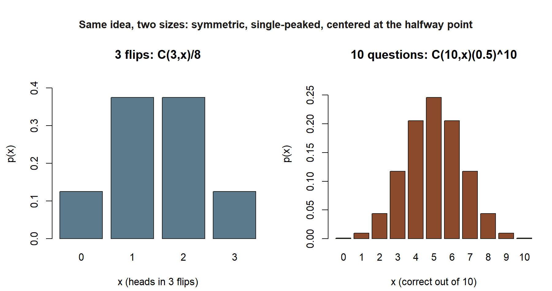
If you want to see a pmf rather than only compute it, the chunk below shows how a student could simulate many quizzes and compare the empirical proportions to \(p(x)\). It is shown for teaching and not run in this build; run it in your own R session.
A common mistake
The mistake to watch for this week is confusing the random variable \(X\) with a value \(x\) it can take, and the related slip of mishandling the integer boundary in the cdf.
The first half: \(X\) is the rule — the capital letter, the whole machine that turns any outcome into a number, with an entire distribution attached. A lowercase \(x\) is one specific number it can land on. Writing “\(P(X)\)” with no value is meaningless; you must say which value, as in \(P(X=3)\), or which range, as in \(P(X\le 2)\). Likewise, \(p(x)\) for a single \(x\) is one probability, while the pmf as a whole is the function across all \(x\). Keep the capital/lowercase distinction crisp and most of the confusion evaporates.
The second half bites in tail probabilities. Because the cdf \(F(x)=P(X\le x)\) includes the mass at \(x\), the two events “\(X>a\)” and “\(X\ge a\)” are not the same for an integer-valued variable. The correct complements are \(P(X>a)=1-F(a)\) but \(P(X\ge a)=1-F(a-1)\). On the quiz, \(P(X\ge 8)\) uses \(1-F(7)\), giving the \(56/1024\approx 0.0547\) above; using \(1-F(8)\) would wrongly drop the mass at \(x=8\). When a tail probability comes out “almost right but a little off,” check this boundary first.
Low-stakes self-checks (ungraded)
These are for your own practice — nothing here is collected or graded.
- For Maya’s quiz, write \(P(X=5)\) as a binomial coefficient over \(1024\), then as a decimal. Is it the single largest value in the pmf? Why does symmetry make \(p(4)=p(6)\)?
- Using the three-flip coin, confirm that the four pmf values sum to \(1\), then state \(P(X=1)\) in words (“the probability of exactly one head”) and check it equals \(3/8\).
- From the coin cdf, compute \(P(1 < X \le 3)\) as \(F(3)-F(1)\). Does it match \(p(2)+p(3)\) directly?
- Explain in one sentence why \(F(x)\) can never go down as \(x\) increases. What would a decrease imply about some \(p(x)\)?
- A small support: let \(Y\) be the number of late shuttles Maya catches in two independent mornings, where each morning is late with probability \(0.19\). Write the support of \(Y\), and set up (do not finish) the pmf for \(Y=0\), \(Y=1\), \(Y=2\) by counting the ways. (We will finish exactly this kind of pmf in Week 9.)
Reading and source pointer
For this week’s spine, read Grinstead & Snell, Chapter 1 (Discrete probability distributions) for the definition of a random variable and its distribution, and Chapter 5 (Important distributions) for how a specific counting pmf — like our quiz’s \(\binom{10}{x}(1/2)^{10}\) — gets recognized as a named distribution. The free online text is at https://www.dartmouth.edu/~chance/teaching_aids/books_articles/probability_book/book.html.
No MIT 18.05 pointer this week; the named-model and simulation strands where 18.05 is genuinely used arrive in Weeks 9 and 13.
These notes are the course’s own synthesis, grounded in but not copied from the sources.
Public vs. graded
These notes, the examples, and the practice here are public and ungraded — study material only. No graded prompts, answer keys, rubrics, point values, or due dates appear on this site. Graded checkpoints, quizzes, homework, labs, the midterm, the project, and the final live in Blackboard (the LMS), which is authoritative for due dates, submissions, and grades. If this page and Blackboard ever disagree, follow Blackboard.
As a preparation note only: this week sits at the course’s midpoint, and the midterm is Friday, October 9, in class, covering the first half of the term — the probability-model, sample-space, conditional-probability, independence, Bayes, counting, and now random-variable material of Weeks 1 through 7 or so. Treat that purely as orientation for how to pace your review. The official scope, format, timing, and everything that counts toward your grade live in Blackboard, which is authoritative; nothing on this public page sets or changes any graded contract.
Looking ahead
You now have a random variable, its pmf, and its cdf — the full description of a discrete number’s behavior. Week 8 asks the two summary questions every distribution invites: where is its center (the expectation \(E[X]=\sum_x x\,p(x)\)) and how spread out is it (the variance \(\operatorname{Var}(X)\) and standard deviation \(\sigma\))? We will compute both for exactly the quiz variable you built today and find its center sits at \(5\) and its spread at \(2.5\) — confirming the “guessing lands near half-right” hunch from the pmf. Week 9 then notices that the quiz pmf, the coin pmf, and many others share one shape, gives that shape its name — the binomial — and adds the Poisson for counts like shuttle arrivals. The “outcome in, number out, probability attached” habit you build this week is the foundation for all of it.
See also
- The notation glossary, for the capital-\(X\)-versus-lowercase-\(x\) and \(p(x)=P(X=x)\) conventions used above: ../resources/notation-glossary.qmd.
- The distribution reference, for how this week’s counting pmf becomes a named model: ../resources/distribution-reference.qmd.
- Where the counting that powers this week’s pmf was built: week-06-counting-and-discrete-probability.qmd.
- Where the pmf’s center and spread are computed next: week-08-expectation-and-variance.qmd.
- Where this pmf earns its name and the binomial/Poisson models arrive: week-09-common-discrete-models.qmd.
- The course syllabus, for the term’s structure and the authoritative pointer to Blackboard: ../syllabus.qmd.