set.seed(35003)
# Synthetic: blind guessing on a 10-question true/false quiz, p = 0.5.
n_trials <- 100000
x <- rbinom(n_trials, size = 10, prob = 0.5)   # number correct, X ~ Binomial(10, 0.5)

mean(x)                       # estimates E[X]  -> near 5
var(x)                        # estimates Var(X) -> near 2.5  (R's var divides by n-1; close at large n)
sd(x)                         # estimates sigma  -> near 1.58

# Same numbers from the exact pmf, for comparison:
xs  <- 0:10
pmf <- dbinom(xs, size = 10, prob = 0.5)
EX  <- sum(xs * pmf)                       # 5
EX2 <- sum(xs^2 * pmf)                      # 27.5
EX                                          # E[X]
EX2 - EX^2 # Var(X) = E[X^2] - (E[X])^2 = 2.5Week 8 — Expectation & variance
Long-run average and spread of a random variable
Mathematical goal
By the end of this week you should be able to take any discrete random variable whose probability mass function you already have and produce two summary numbers from it — its expectation and its variance — and say in plain words what each one measures. Concretely, the week’s targets are:
- the definition of expectation, \(E[X]=\sum_x x\,p(x)\), read as the long-run average value of \(X\);
- the computational formula for variance, \(\operatorname{Var}(X)=E[X^2]-\big(E[X]\big)^2\), read as the average squared distance of \(X\) from its own mean, together with the standard deviation \(\sigma=\sqrt{\operatorname{Var}(X)}\) that puts spread back on the original scale;
- the two linearity / rescaling rules, \(E[aX+b]=aE[X]+b\) and \(\operatorname{Var}(aX+b)=a^2\operatorname{Var}(X)\);
- and the skill of getting the same answer two ways — straight from the definition, and from a known formula like \(E[X]=np\) for a binomial count — so that a clean shortcut and a first-principles sum confirm each other.
This is a derivation week, so the emphasis is on where the formulas come from and why they are allowed, not just on plugging numbers into them. All worked numbers are synthetic (seed 35003 set) and held fixed.
The week question
Last week you learned to describe a discrete random variable completely with its pmf \(p(x)\) — a full table of every value and its probability. That is the honest, complete answer to “what does \(X\) do?” But a full table is a lot to carry around, and most real decisions only need a couple of summary numbers. So this week asks:
If we already know the whole probability mass function of \(X\), what single number best captures its typical value, and what single number best captures how much it tends to vary around that typical value? And once we have those, how do they change if we rescale or shift \(X\) — say, convert correct-answers to a point score, or minutes to hours?
The “typical value” question is answered by expectation; the “how much it varies” question is answered by variance and its square root, the standard deviation. The rescaling question is answered by the two linearity rules. We will derive each from the pmf and then test them on the running quiz-guessing case.
Notation
| Symbol | Meaning |
|---|---|
| \(X,\,Y\) | random variables (capitals); their values are lowercase \(x,y\) |
| \(p(x)=P(X=x)\) | probability mass function — the probability \(X\) takes the value \(x\) |
| \(E[X]\) | expectation (mean) of \(X\); written \(\mu\) when we name the resulting value |
| \(E[X^2]\) | expectation of \(X^2\) — average of the squared values, \(\sum_x x^2 p(x)\) |
| \(E[g(X)]\) | expectation of a function of \(X\), \(\sum_x g(x)\,p(x)\) |
| \(\operatorname{Var}(X)=\sigma^2\) | variance of \(X\) — average squared distance from the mean |
| \(\sigma=\sqrt{\operatorname{Var}(X)}\) | standard deviation — spread on the original scale of \(X\) |
| \(a,\,b\) | constants used to rescale (\(a\)) and shift (\(b\)) a random variable |
| \(n,\,p\) | for a binomial count: number of trials and per-trial success probability |
| \(X\sim\text{Binomial}(n,p)\) | “\(X\) is distributed as a binomial count of successes in \(n\) trials” |
Two reminders carried in from earlier weeks: \(p(x)\) is a genuine probability (it lives in \([0,1]\) and the \(p(x)\) over the support sum to \(1\)), and the support is just the list of values \(x\) where \(p(x)>0\). Every sum \(\sum_x\) below runs over that support.
Conceptual setup
Expectation as a probability-weighted average. Imagine watching \(X\) over a very long run of independent repetitions and recording every value it takes. The arithmetic average of those records does not weight every possible value equally — it weights each value by how often it shows up, which is exactly \(p(x)\). Pushing that long-run average to its limit gives the definition
\[ E[X] \;=\; \sum_x x\,p(x). \]
So \(E[X]\) is a weighted average of the values, with the probabilities as weights. It need not be a value \(X\) can actually take (the average of a fair die, as we will see, is \(3.5\)), and it is a parameter of the distribution, not a statistic computed from a finite sample — a distinction we will lean on hard in Week 13.
Functions of \(X\), and \(E[X^2]\). If \(g\) is any function, then \(g(X)\) is itself a random variable, and its expectation is obtained by weighting the transformed values by the same probabilities:
\[ E[g(X)] \;=\; \sum_x g(x)\,p(x). \]
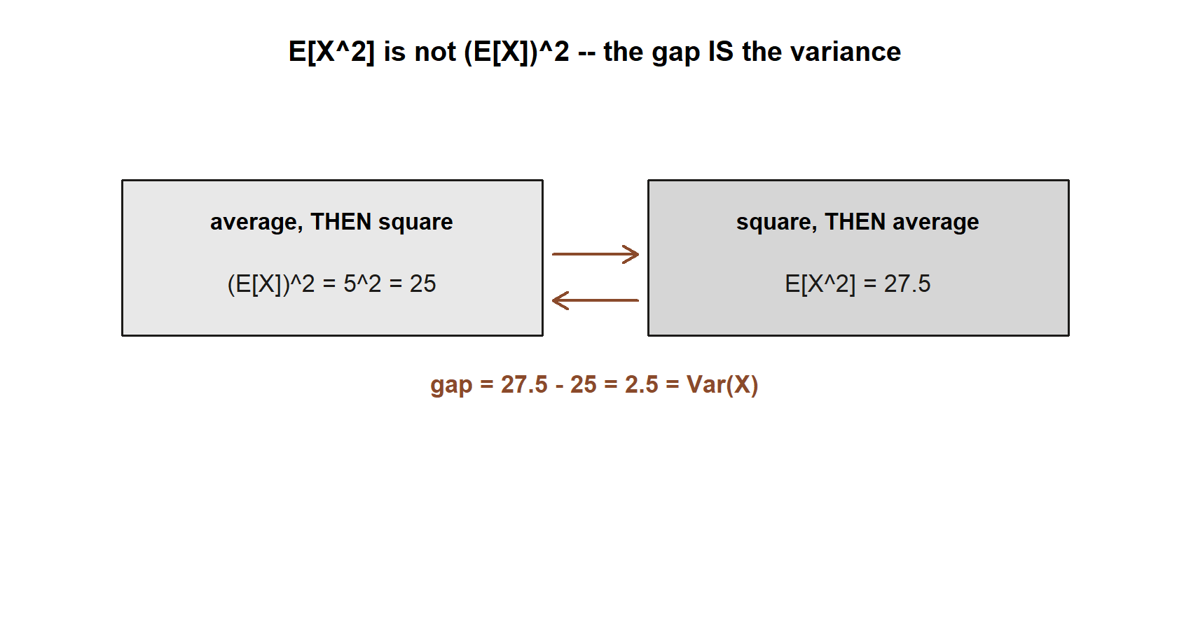
The case \(g(x)=x^2\) gives \(E[X^2]=\sum_x x^2 p(x)\). Note carefully that \(E[X^2]\) is generally not equal to \(\big(E[X]\big)^2\) — you square then average, which is different from averaging then squaring. That very gap is what variance measures.
Variance as average squared distance from the mean. A natural way to measure spread is “how far is \(X\), on average, from its own mean \(\mu=E[X]\)?” Plain distance \(X-\mu\) averages to zero (the positive and negative deviations cancel), so we average the squared deviation instead:
\[ \operatorname{Var}(X) \;=\; E\big[(X-\mu)^2\big] \;=\; \sum_x (x-\mu)^2\,p(x). \]
This is always \(\ge 0\), and it is \(0\) only when \(X\) is a constant. Expanding the square and using linearity of the sum turns this into the computational formula we will actually use:
\[ \operatorname{Var}(X) = E\big[X^2 - 2\mu X + \mu^2\big] = E[X^2] - 2\mu\,E[X] + \mu^2 = E[X^2] - 2\mu^2 + \mu^2 = E[X^2] - \mu^2, \]
that is, \(\boxed{\operatorname{Var}(X)=E[X^2]-\big(E[X]\big)^2.}\) The first form (\(\sum (x-\mu)^2 p(x)\)) shows what variance means; the second form (\(E[X^2]-\mu^2\)) is what you compute, since it needs only two sums. Because variance is in squared units, we report spread on the original scale with the standard deviation \(\sigma=\sqrt{\operatorname{Var}(X)}\).
The two rescaling rules. Suppose we build a new variable \(Y=aX+b\) by stretching \(X\) by a factor \(a\) and sliding it by a constant \(b\). Two facts follow directly from the definitions:
\[ E[aX+b] \;=\; a\,E[X]+b, \qquad \operatorname{Var}(aX+b) \;=\; a^2\,\operatorname{Var}(X). \]
For the mean, the additive constant \(b\) moves the average by exactly \(b\), and the multiplier \(a\) scales it by \(a\) — average and arithmetic commute. For the variance, the shift \(b\) does not change spread at all (sliding every value left or right leaves the gaps between them untouched), and the stretch \(a\) scales every deviation by \(a\), hence the squared deviation by \(a^2\). On the standard-deviation scale this reads \(\sigma_{aX+b}=|a|\,\sigma_X\) — the absolute value because a negative \(a\) flips the variable but spread is never negative.
Worked example
We work the recurring quiz-guessing case symbolically first, then numerically, and confirm each summary number two independent ways. Then a fresh transfer example — a single die roll — exercises the same machinery in a new context. Data are synthetic; seed 35003 set.
The recurring slice — guessing a 10-question true/false quiz
Maya answers a 10-question true/false quiz by pure guessing, so each question is an independent success with probability \(p=0.5\), and \(X\) is the number she gets correct. From Weeks 6–7 we already have the model \(X\sim\text{Binomial}(n,p)\) with \(n=10\), \(p=0.5\), and pmf \(p(x)=\binom{10}{x}(0.5)^{10}\) on the support \(\{0,1,\dots,10\}\).
Expectation, symbolically. Rather than grind out the ten-term sum \(\sum_{x=0}^{10} x\binom{10}{x}(0.5)^{10}\), think of \(X\) as a sum of per-question indicators. Let \(X_i=1\) if question \(i\) is correct and \(0\) otherwise, so \(X=X_1+\cdots+X_{10}\). Each indicator has \(E[X_i]=1\cdot p + 0\cdot(1-p)=p\). By linearity of expectation (the additive rule applied \(n\) times),
\[ E[X] = E\!\left[\sum_{i=1}^{n} X_i\right] = \sum_{i=1}^{n} E[X_i] = \sum_{i=1}^{n} p = n\,p. \]
So for any binomial count \(E[X]=np\).
Expectation, numerically — two ways. The formula gives
\[ E[X] = n\,p = 10\times 0.5 = 5. \]
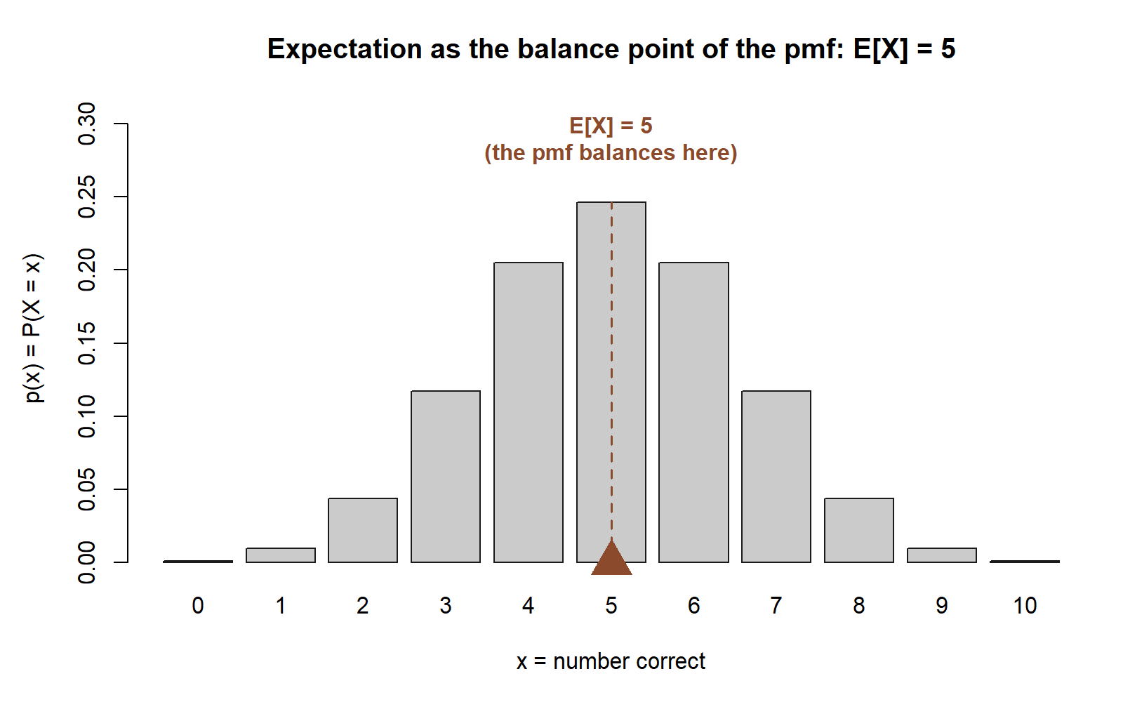
As a check, the symmetry of the pmf does the same job: \(p(x)=p(10-x)\), so the distribution is mirror-symmetric about \(x=5\), and a symmetric distribution’s mean sits exactly at its center of symmetry — again \(E[X]=5\). Both routes agree: \(E[X]=5\). On average, blind guessing earns five correct out of ten — reassuringly, half.
Variance, symbolically. For a binomial count the same indicator decomposition (with the per-question variance \(\operatorname{Var}(X_i)=p(1-p)\), and independence letting the variances add — a fact we will prove in Week 12) gives the standard result
\[ \operatorname{Var}(X) = \sum_{i=1}^{n}\operatorname{Var}(X_i) = n\,p(1-p). \]
We will also get the same number straight from the definition \(\operatorname{Var}(X)=E[X^2]-(E[X])^2\), to show the general machinery and the shortcut land in the same place.
Variance, numerically — two ways. The binomial formula gives
\[ \operatorname{Var}(X) = n\,p(1-p) = 10\times 0.5 \times 0.5 = 2.5. \]
Now the definition route. We already have \(\mu=E[X]=5\), so we need \(E[X^2]=\sum_x x^2 p(x)\). There is a clean identity for it: \(E[X^2]=\operatorname{Var}(X)+\mu^2\), but using that would be circular here, so instead use \(E[X^2]=E[X(X-1)]+E[X]\) together with the binomial factorial-moment fact \(E[X(X-1)]=n(n-1)p^2\). For \(n=10,\ p=0.5\),
\[ E[X(X-1)] = n(n-1)p^2 = 10\cdot 9 \cdot 0.25 = 22.5, \qquad E[X^2] = 22.5 + 5 = 27.5. \]
Then the computational formula gives
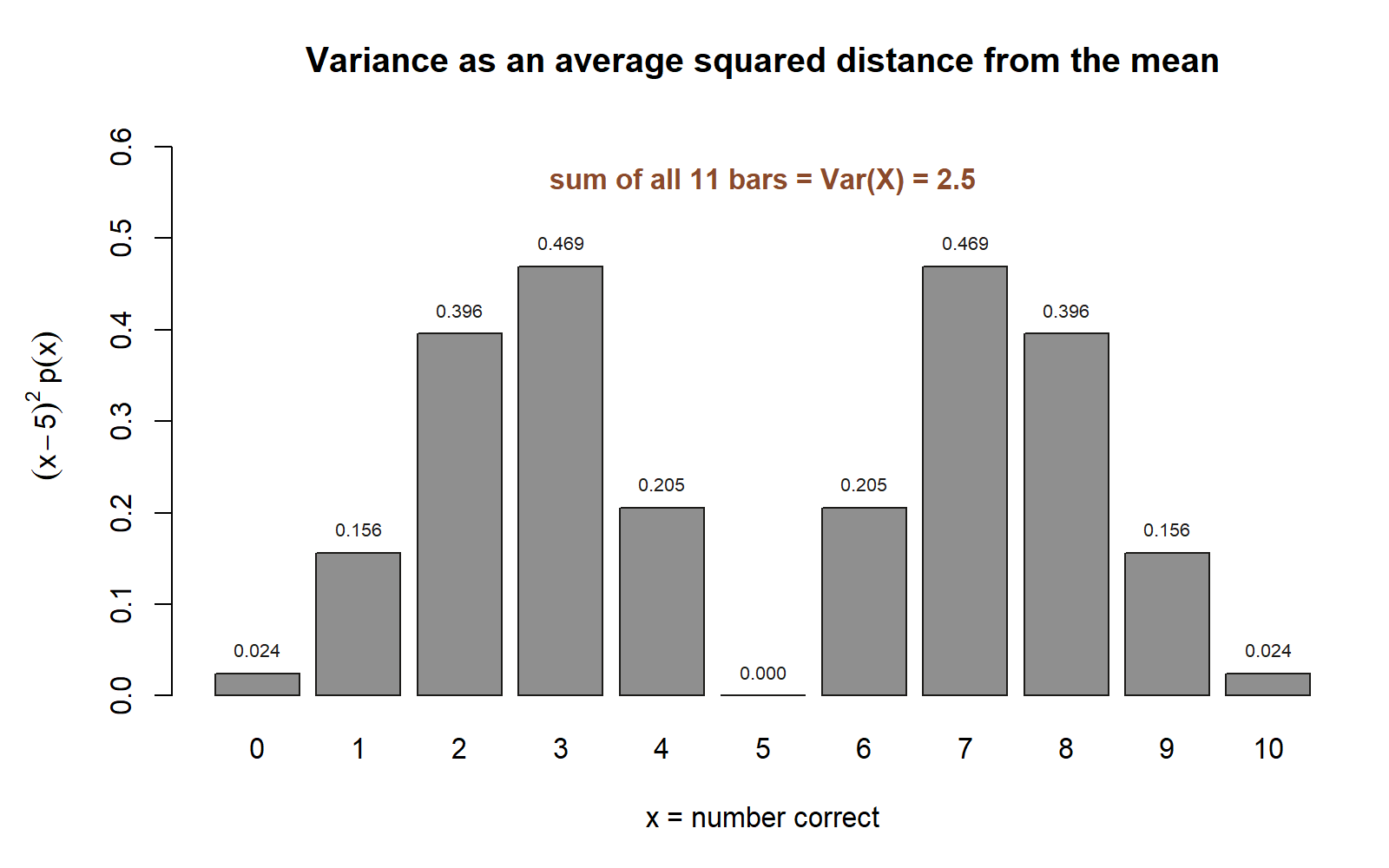
\[ \operatorname{Var}(X) = E[X^2]-\big(E[X]\big)^2 = 27.5 - 5^2 = 27.5 - 25 = 2.5. \]
The definition route and the \(np(1-p)\) shortcut agree exactly: \(\operatorname{Var}(X)=2.5\). The standard deviation puts that spread back on the “number-correct” scale:
\[ \sigma = \sqrt{\operatorname{Var}(X)} = \sqrt{2.5} \approx 1.58. \]
So a blind guesser scores about \(5\) correct, give or take roughly \(1.58\) — a compact, decision-ready summary of the whole 11-row pmf.
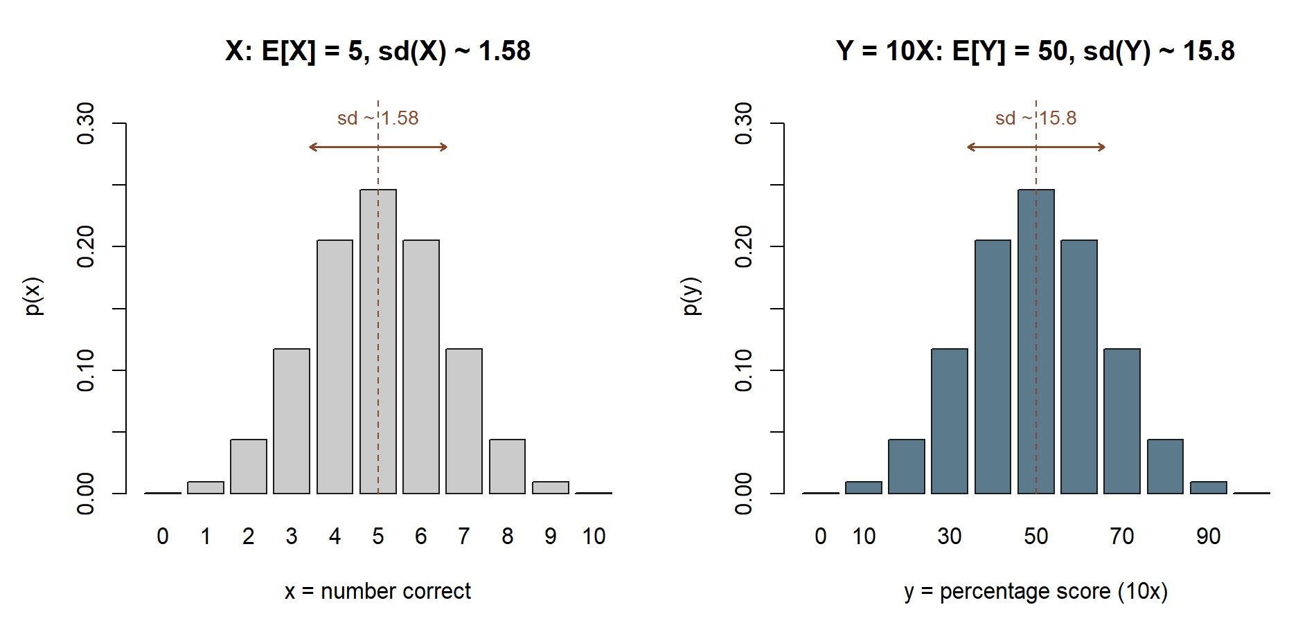
Rescaling, in context. Suppose the quiz is reported as a percentage score \(Y=10X\) (ten points per question). The rules predict the summaries without redoing any sum:
\[ E[Y] = E[10X] = 10\,E[X] = 50, \qquad \operatorname{Var}(Y) = \operatorname{Var}(10X) = 10^2\,\operatorname{Var}(X) = 100\times 2.5 = 250, \]
so \(\sigma_Y = 10\,\sigma_X \approx 15.8\) percentage points. If instead each student were handed two free points, \(Y=X+2\), the mean would rise to \(7\) but the variance would stay at \(2.5\) — a shift moves the center, never the spread.
You can see the same two summaries by simulation; the chunk below is shown for teaching and is not run in this build. Run it in your own R session and the seed makes the result reproducible.
Transfer example — the average of a single fair die roll
Now apply the same definitions in a brand-new context. Let \(D\) be the result of one roll of a fair six-sided die, so the support is \(\{1,2,3,4,5,6\}\) with \(p(d)=\tfrac{1}{6}\) for each face. (Synthetic; seed 35003 set.)
Expectation from the definition.
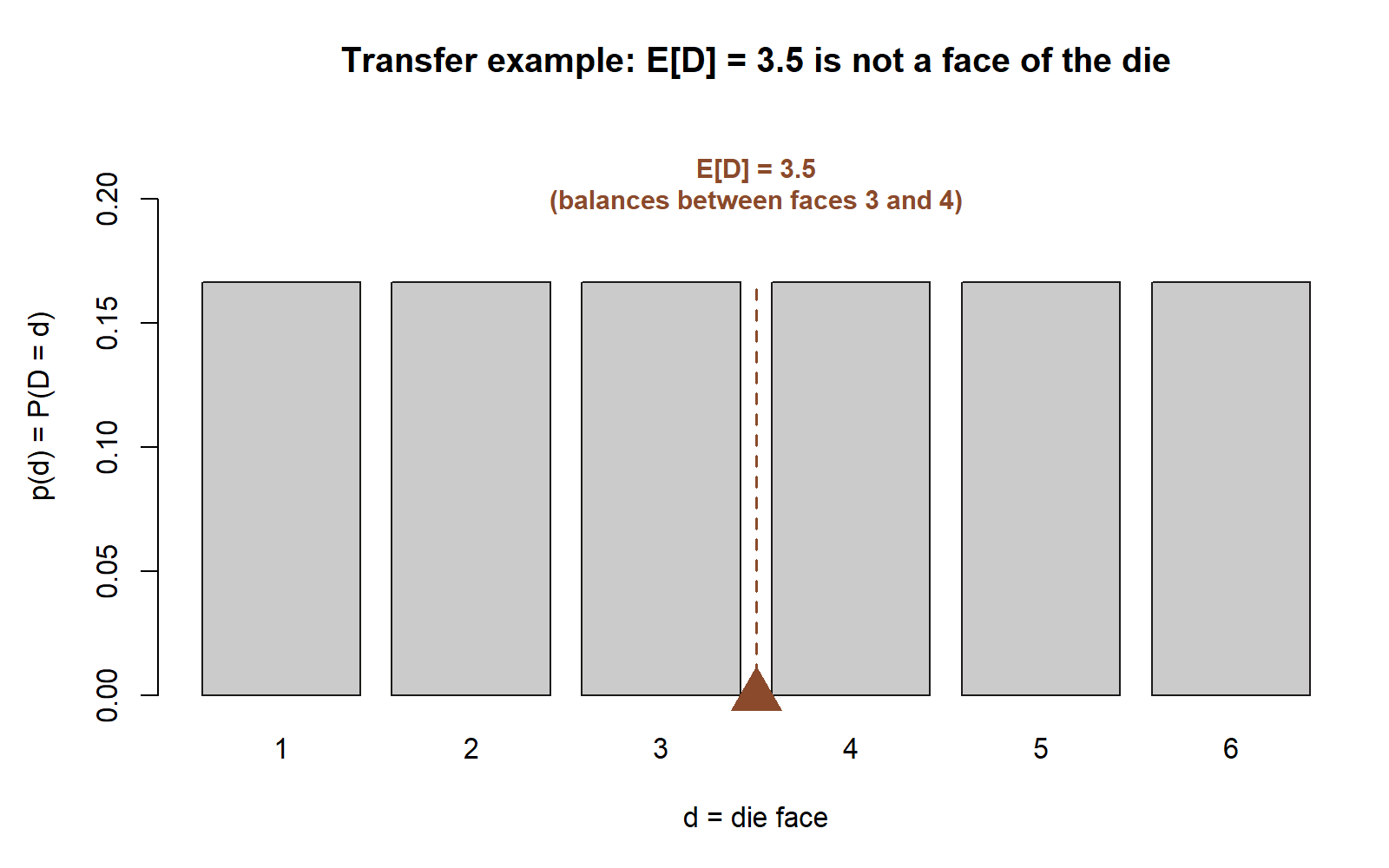
\[ E[D] = \sum_{d=1}^{6} d\cdot\tfrac{1}{6} = \tfrac{1}{6}(1+2+3+4+5+6) = \tfrac{21}{6} = 3.5. \]
The “expected” value \(3.5\) is not a face the die can show — it is the long-run average, sitting exactly at the midpoint of the symmetric set of faces, just as the quiz mean sat at the symmetry center \(5\).
Variance from the computational formula. First the second moment,
\[ E[D^2] = \sum_{d=1}^{6} d^2\cdot\tfrac{1}{6} = \tfrac{1}{6}(1+4+9+16+25+36) = \tfrac{91}{6}, \]
then
\[ \operatorname{Var}(D) = E[D^2]-\big(E[D]\big)^2 = \tfrac{91}{6} - (3.5)^2 = \tfrac{91}{6} - \tfrac{49}{4} = \tfrac{182-147}{12} = \tfrac{35}{12} \approx 2.92, \]
with standard deviation \(\sigma_D=\sqrt{35/12}\approx 1.71\). Notice the die — six equally-likely faces — is slightly more spread out (\(\approx 2.92\)) than the quiz count (\(2.5\)), which makes sense: the quiz piles probability up near its center, while the die spreads it evenly across its range. Same two formulas, a new distribution, fully consistent answers.
A convention warning
A few places where the algebra quietly bites, all on this week’s convention-risk list:
- \(\sigma^2\) and \(\operatorname{Var}(X)\) are the same object. We use both notations interchangeably: \(\operatorname{Var}(X)\) when we want to name the operation, \(\sigma^2\) when we want a compact symbol, and \(\sigma=\sqrt{\operatorname{Var}(X)}\) for the standard deviation. They are defined once and identical — do not read \(\sigma^2\) as a different quantity from the variance.
- \(E[X^2]\ne\big(E[X]\big)^2\). Squaring and averaging do not commute; their difference is precisely \(\operatorname{Var}(X)\), which is why it is non-negative. Writing \(E[X^2]=(E[X])^2\) silently forces every variance to zero — a classic and costly slip. In the quiz case the two are \(27.5\) versus \(25\), and that gap of \(2.5\) is the variance.
- The variance rule has \(a^2\), not \(a\), and ignores \(b\). \(\operatorname{Var}(aX+b)=a^2\operatorname{Var}(X)\): the multiplier enters squared (because it scales a squared deviation), and the additive shift \(b\) drops out entirely (sliding the whole distribution does not change its spread). Forgetting the square, or letting \(b\) leak into the variance, are the two most common errors here.
- Variance is in squared units; report spread with \(\sigma\). The quiz variance \(2.5\) is in “(correct-answers)\(^2\),” which is not interpretable on its own. Take the square root to get \(\sigma\approx 1.58\) correct answers before you talk about typical spread.
- \(E[X]\) need not be attainable. A mean of \(5\) correct or \(3.5\) pips is a long-run average, not a guaranteed or even possible single outcome. Read it as “the balance point of the distribution,” not “what will happen.”
Practice (ungraded)
Work these for yourself; they are ungraded self-checks, not submissions. Each should fall straight out of this week’s definitions and rules — no new machinery needed.
- A small synthetic random variable has \(p(0)=0.5,\ p(1)=0.3,\ p(2)=0.2\). Compute \(E[X]\) from the definition, then \(E[X^2]\), then \(\operatorname{Var}(X)=E[X^2]-(E[X])^2\) and \(\sigma\). Check your \(E[X]\) lies between the smallest and largest values.
- For the guessing quiz (\(X\sim\text{Binomial}(10,0.5)\)), reconstruct \(E[X]=5\) and \(\operatorname{Var}(X)=2.5\) both ways — once from \(np\) and \(np(1-p)\), and once from the definition via \(E[X^2]-\mu^2\) — and confirm the two routes match.
- The percentage score is \(Y=10X\). Without summing anything, use the rescaling rules to write down \(E[Y]\), \(\operatorname{Var}(Y)\), and \(\sigma_Y\) from the quiz summaries. Then handle the “two free points” version \(Y=X+2\): which of the three summaries changes, and which does not?
- Re-derive the fair-die summaries \(E[D]=3.5\) and \(\operatorname{Var}(D)=35/12\approx 2.92\) from the definitions, and confirm \(\sigma_D=\sqrt{35/12}\). Then predict, using a rescaling rule only, the expectation and variance of \(2D\) (rolling and doubling).
- Reasoning check, no computation: explain in one or two sentences why adding a constant to every value of a random variable cannot change its variance, but multiplying every value by \(3\) multiplies the variance by \(9\).
Reading and source pointer
For this week, read Grinstead & Snell, Introduction to Probability, Chapter 6 — Expected Value and Variance, the free online text: https://www.dartmouth.edu/~chance/teaching_aids/books_articles/probability_book/book.html. That chapter develops expectation, the variance of a discrete random variable, and the algebra of how both behave under scaling and shifting — the same scaffold this note builds, in the same order. (No MIT 18.05 pointer is assigned this week; it returns in Week 9 with the standard discrete models.)
These notes are the course’s own synthesis, grounded in but not copied from the sources. All examples and numbers here are original and synthetic (seed 35003 set); none are taken from the text’s examples, exercises, figures, or solutions.
Public vs. graded
These notes, the examples, and the practice here are public and ungraded — study material only. No graded prompts, answer keys, rubrics, point values, or due dates appear on this site. Graded checkpoints, quizzes, homework, labs, the midterm, the project, and the final live in Blackboard (the LMS), which is authoritative for due dates, submissions, and grades. If this page and Blackboard ever disagree, follow Blackboard.
Looking ahead
You now have two summary numbers — mean and variance — for any discrete random variable, plus the rules for how they move under rescaling. Next week we stop building summaries by hand for ad-hoc pmfs and instead meet the common discrete models that come with their means and variances already worked out: the binomial we have been leaning on (so \(E[X]=np\) and \(\operatorname{Var}(X)=np(1-p)\) become named facts, not re-derivations), the geometric, and the Poisson model for the shuttle-arrivals thread. The expectation and variance machinery from this week is exactly the lens we will use to read each of those models.
See also
- Week 7 — Discrete random variables — where the quiz pmf \(p(x)=\binom{10}{x}(0.5)^{10}\) comes from; this week summarizes that pmf.
- Week 9 — Common discrete models — the binomial, geometric, and Poisson models that package these summaries as named formulas.
- Notation glossary — the binding symbols for \(E[X]\), \(\operatorname{Var}(X)=\sigma^2\), \(\sigma\), and the rescaling rules.
- Distribution reference — quick mean/variance facts for the standard models, with parameterizations fixed.
- Course syllabus — schedule, policies, and where graded work lives.