Week 6 — Counting & discrete probability

Counting outcomes when equally-likely models are reasonable

The week question

When every outcome of an experiment is equally likely, a probability is just a fraction: how many outcomes make the event happen, divided by how many outcomes there are in total. That sounds easy — and for a single coin or a single die it is. But the moment the experiment has any structure to it — ten coin flips in a row, a committee chosen from a club, the letters of a word rearranged — the two counts get large fast, and counting them one-by-one stops working. So this week’s question is a counting question dressed up as a probability question:

How do we count the number of outcomes in a structured experiment, so that we can turn an equally-likely model into an actual probability?

We build three tools — the multiplication principle, permutations, and combinations — and then we point them at the running example that will carry us through the next several weeks: a student guessing on a ten-question true/false quiz.

Why this matters

Almost every probability you will ever compute “by hand” in this course rests on one of two foundations. The first is the equally-likely model: when symmetry makes it reasonable to treat every outcome the same, \(P(E)\) is the number of outcomes in \(E\) divided by the number of outcomes in the whole sample space. The second, which we meet later, is a named distribution. This week is about the first foundation, and counting is its raw material — without a reliable way to count outcomes, an equally-likely model is just a promise you cannot cash.

Counting also quietly powers the binomial distribution, which becomes the spine of Weeks 7 through 9. When we ask “how many ways can a guessing student get exactly \(5\) of \(10\) questions right?”, the answer is a combination, \(\binom{10}{5}\). The pmf we write in Week 7, the expectation and variance we derive in Week 8, and the binomial model we name in Week 9 are all built on the counts you learn to produce here. Getting comfortable with \(n!\), \(\frac{n!}{(n-k)!}\), and \(\binom{n}{k}\) now means those later weeks are about ideas, not arithmetic surprises.

Learning goals

By the end of this week you should be able to:

• State the multiplication principle and use it to count the outcomes of a multi-stage experiment.
• Distinguish ordered counting (permutations) from unordered counting (combinations), and choose the right one by asking whether order changes the outcome.
• Compute a permutation \(\frac{n!}{(n-k)!}\) and a combination \(\binom{n}{k}=\frac{n!}{k!\,(n-k)!}\) for small \(n\) and \(k\), by hand and with R.
• Turn a count into an equally-likely probability by dividing the favorable count by the total count.
• Explain why the ten-question true/false quiz has \(2^{10}=1024\) equally-likely answer keys, and why the number with exactly \(k\) correct is \(\binom{10}{k}\).

Core vocabulary

• Multiplication principle. If a process happens in stages, and stage one can occur in \(n_1\) ways, stage two in \(n_2\) ways, and so on independently of how earlier stages turned out, then the whole process can occur in \(n_1\times n_2\times\cdots\) ways.
• Factorial. \(n! = n\times(n-1)\times\cdots\times 2\times 1\) counts the arrangements of \(n\) distinct items in a row. By convention \(0!=1\).
• Permutation. An ordered selection of \(k\) items from \(n\) distinct items. There are \(\frac{n!}{(n-k)!}\) of them. Order matters: ABC and ACB are different permutations.
• Combination. An unordered selection of \(k\) items from \(n\) distinct items. There are \(\binom{n}{k}=\frac{n!}{k!\,(n-k)!}\) of them. Order is ignored: \(\{A,B,C\}\) and \(\{A,C,B\}\) are the same combination.
• Equally-likely model. A sample space \(\Omega\) in which every outcome carries probability \(1/|\Omega|\), so that \(P(E)=|E|/|\Omega|\) for any event \(E\). This is a modeling choice, justified by symmetry, not a law of nature.

(All scenario data this week are synthetic; seed 35003 set.)

Concept development

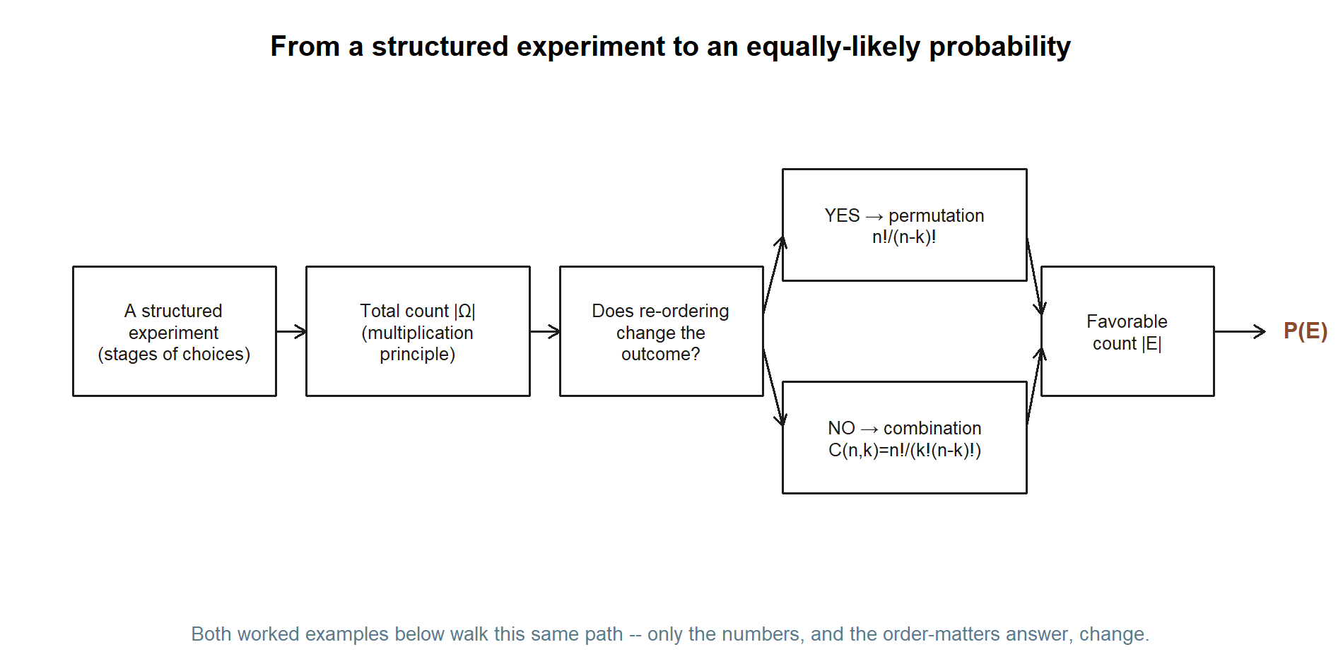
Before building the three tools one at a time, it helps to see the whole route from “a structured experiment” to “an actual probability” laid out as a single path. Every worked example below — the quiz, the committee, the officer slate — walks this exact path; only the numbers, and the answer to “does order matter?”, change.

Figure 1: The week’s method, end to end (synthetic). A structured experiment first needs a total count \(|\Omega|\) from the multiplication principle; then a single question — does re-ordering the selection change the outcome? — routes you to a permutation or a combination for the favorable count \(|E|\); dividing gives \(P(E)=|E|/|\Omega|\).

What the figure shows (non-visual equivalent). Five steps, always in this order: (1) count everything with the multiplication principle, (2) ask whether reordering the selection changes the outcome, (3a) if yes, count with a permutation, or (3b) if no, count with a combination, (4) that count is the favorable count \(|E|\), and (5) \(P(E)=|E|/|\Omega|\). Synthetic instructional example; numbers are illustrative.

The multiplication principle: counting in stages

Most interesting experiments are not single actions; they are sequences of smaller actions. The multiplication principle is the engine that turns “a sequence of choices” into a single count. If you make a first choice in \(n_1\) ways and, no matter what you chose first, a second choice in \(n_2\) ways, then together you have \(n_1 \times n_2\) ways.

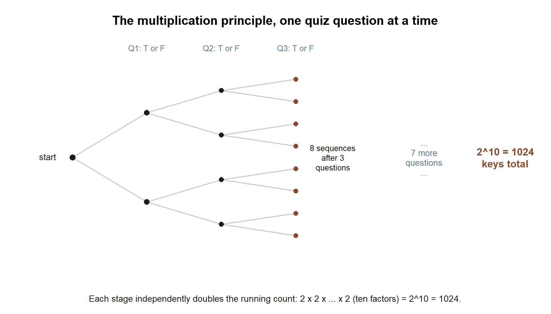
The “no matter what you chose first” clause is the part to watch. The principle works cleanly when the number of options at each stage does not depend on the earlier outcomes. Tossing a fair coin ten times is the canonical case: each toss has \(2\) outcomes regardless of what came before, so a full sequence of ten tosses is one of

\[ \underbrace{2\times 2\times\cdots\times 2}_{10\text{ factors}} = 2^{10} = 1024 \]

equally-likely sequences. The same logic counts the answer keys of a ten-question true/false quiz: each question is independently True or False, so there are \(2^{10}=1024\) possible keys. We will lean on exactly this count in the worked examples.

Drawing the first few stages as a tree makes the doubling pattern concrete before you trust it out to ten questions.

Figure 2: Counting in stages, one branch at a time (synthetic). The first three questions of the quiz, drawn as a tree: each True/False question doubles the number of branches, giving \(2\times2\times2=8\) sequences after three questions. The same doubling continues through all ten questions.

What the figure shows (non-visual equivalent). Each level of the tree doubles the branch count: \(2\), then \(4\), then \(8\) after three questions. Continuing the same doubling seven more times gives \(2^{10}=1024\) — the multiplication principle is exactly this repeated doubling, just too wide to draw past a few stages. Synthetic instructional example; numbers are illustrative.

Permutations: when order is part of the outcome

Sometimes the order of a selection is itself part of what we are counting. Lining up \(n\) distinct people for a photo, or filling the distinct roles of president, secretary, and treasurer, are ordered problems: swapping two people produces a genuinely different arrangement.

Arranging all \(n\) distinct items in a row is a direct application of the multiplication principle. The first slot has \(n\) choices, the second has \(n-1\) (one item is used up), and so on down to \(1\):

\[ n\times(n-1)\times\cdots\times 1 = n!. \]

If we only fill \(k\) of the slots — choosing an ordered list of \(k\) items from \(n\) — the product stops after \(k\) factors, which we write compactly as a ratio of factorials:

\[ \frac{n!}{(n-k)!} = \underbrace{n\times(n-1)\times\cdots\times(n-k+1)}_{k\text{ factors}}. \]

This is the number of permutations of \(k\) items chosen from \(n\). The factorial in the denominator simply cancels the slots we never filled.

Combinations: when order does not matter

Very often we want a group, not an ordering. A three-person committee is the same committee no matter the order in which we name its members; a five-card poker hand is the same hand however it is dealt. For these problems, permutations over-count, because they treat every reordering of the same group as distinct.

The fix is to divide out the orderings. A group of \(k\) items can be arranged in \(k!\) ways, so each unordered group of \(k\) corresponds to exactly \(k!\) different ordered selections. Dividing the permutation count by \(k!\) removes that redundancy and gives the number of combinations:

\[ \binom{n}{k} = \frac{1}{k!}\cdot\frac{n!}{(n-k)!} = \frac{n!}{k!\,(n-k)!}. \]

We read \(\binom{n}{k}\) as “\(n\) choose \(k\).” Two facts are worth memorizing because they show up constantly. First, \(\binom{n}{k}=\binom{n}{n-k}\): choosing which \(k\) to include is the same as choosing which \(n-k\) to leave out. Second, \(\binom{n}{0}=\binom{n}{n}=1\): there is exactly one way to choose nothing and exactly one way to choose everything.

From counts to equally-likely probabilities

Once we can count, the equally-likely model is short work. If symmetry makes every outcome in \(\Omega\) equally probable, then for any event \(E\),

\[ P(E) = \frac{|E|}{|\Omega|} = \frac{\text{number of outcomes that make }E\text{ happen}}{\text{total number of outcomes}}. \]

The discipline this imposes is healthy: to find a probability you must answer two clean counting questions — how many outcomes total, and how many favorable. The multiplication principle usually answers the first; permutations or combinations usually answer the second. Choosing between permutations and combinations comes down to a single question you should ask every time: does reordering the selection change the outcome? If yes, count ordered (permutations). If no, count unordered (combinations).

A caution worth stating now: the equally-likely model is a choice, defensible only when the outcomes really are symmetric. A fair coin, a balanced die, and a student guessing with no knowledge all justify it. A loaded die or a student who actually knows some answers does not — for those we need the weighted models of the coming weeks.

Worked examples

Worked example — the recurring slice: counting on the ten-question quiz

Maya’s study group is curious about a familiar fear: if you walked into a ten-question true/false quiz and guessed every answer, how likely is each possible score? This is the quiz-guessing thread we will carry all the way to Week 9, and Week 6 is where we lay its counting foundation. (Synthetic; seed 35003 set.)

Symbolic setup. Each question is answered True or False, so an answer key — the full list of ten responses — is a length-10 sequence of two symbols. By the multiplication principle there are

\[ |\Omega| = 2^{10} = 1024 \]

possible keys. Because the student is guessing with no knowledge, it is reasonable to treat all \(1024\) keys as equally likely. Now fix a score \(k\) (the number of questions answered correctly). An outcome scores exactly \(k\) when the set of questions that happen to be right has size \(k\). The order in which we name those \(k\) questions does not matter — what matters is which \(k\) of the \(10\) are correct — so the number of keys with exactly \(k\) correct is a combination:

\[ |E_k| = \binom{10}{k}. \]

Putting the two counts together gives the equally-likely probability of scoring exactly \(k\):

\[ P(\text{exactly }k\text{ correct}) = \frac{\binom{10}{k}}{2^{10}} = \frac{\binom{10}{k}}{1024}. \]

Numeric instance. Take the middle score, \(k=5\). The favorable count is

\[ \binom{10}{5} = \frac{10!}{5!\,5!} = \frac{10\cdot 9\cdot 8\cdot 7\cdot 6}{5\cdot 4\cdot 3\cdot 2\cdot 1} = \frac{30240}{120} = 252, \]

so

\[ P(\text{exactly }5\text{ correct}) = \frac{\binom{10}{5}}{1024} = \frac{252}{1024} \approx 0.246. \]

Even the single most likely score happens under one in four times — a useful first hint that “guessing your way to a good grade” is a poor plan. As a sanity check, the favorable counts across all scores must add up to the total number of keys, and they do: \(\sum_{k=0}^{10}\binom{10}{k}=2^{10}=1024\). This identity is exactly the multiplication-principle count of all keys, recovered by adding up the by-score counts — a nice internal consistency check, and the seed of the binomial pmf you will write in Week 7.

Seeing all eleven by-score counts side by side, rather than just the one at \(k=5\), shows the whole shape of this counting exercise at a glance.

Figure 3: How the 1024 keys split by score (synthetic). The count \(\binom{10}{k}\) of answer keys with exactly \(k\) correct, for \(k=0,\dots,10\). These are raw counts, not probabilities — dividing each by \(1024\) is what turns this picture into the pmf of Week 7.

What the figure shows (non-visual equivalent). The bars, left to right, are \(1, 10, 45, 120, 210, 252, 210, 120, 45, 10, 1\) — symmetric, tallest at \(k=5\) with \(\binom{10}{5}=252\), and summing to \(1024\). Nothing here is a probability yet; that division happens in Week 7. Synthetic instructional example; numbers are illustrative.

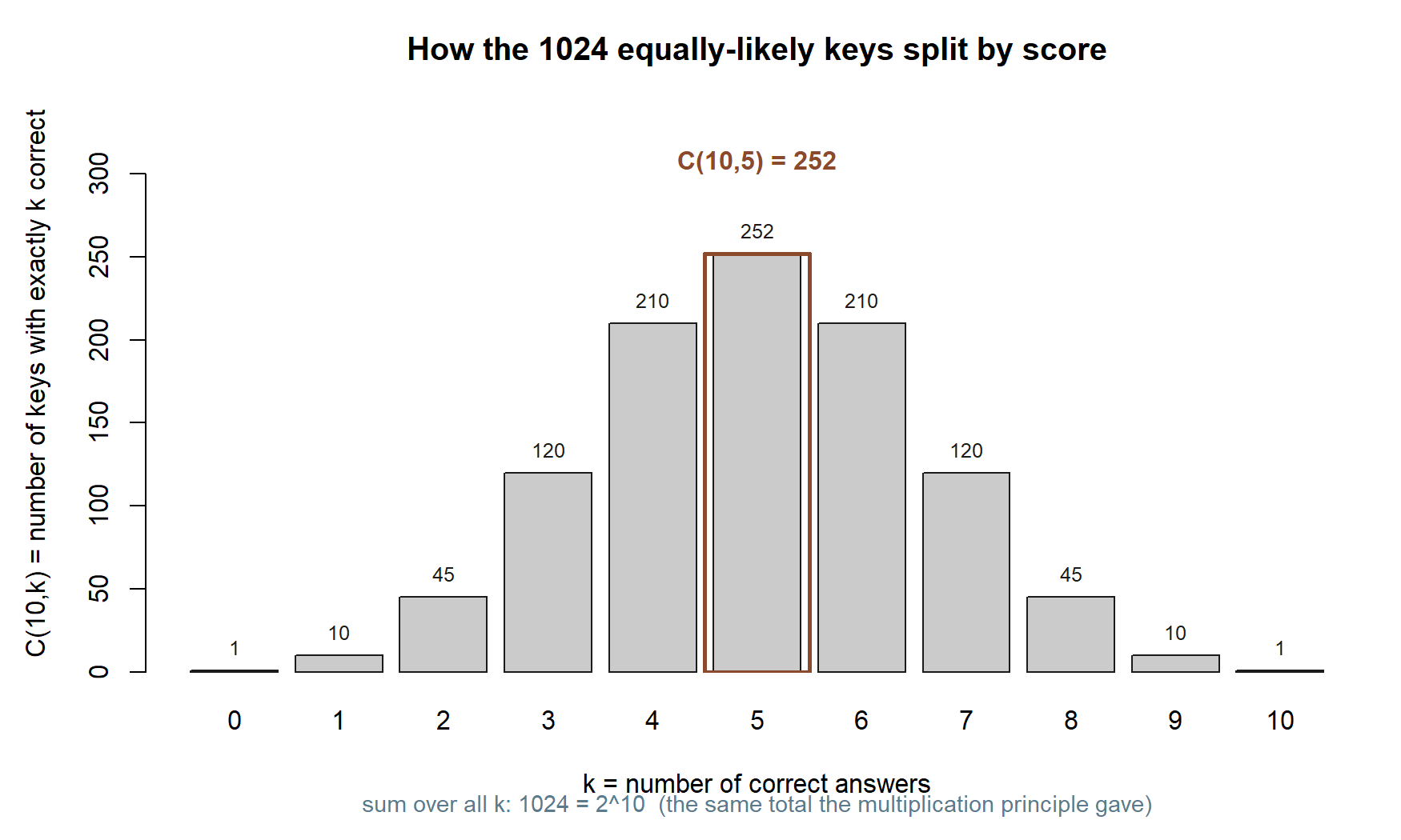
You can reproduce these counts in R. The chunk below is shown as teaching, not executed in this build; run it in your own session to see the numbers.

set.seed(35003)

# Total number of equally-likely answer keys on a 10-question T/F quiz
total_keys <- 2^10                 # 1024

# Number of keys with exactly k correct, for k = 0..10
ways_exactly_k <- choose(10, 0:10) # 1 10 45 120 210 252 210 120 45 10 1

# Probability of exactly 5 correct under pure guessing
p_exactly_5 <- choose(10, 5) / total_keys   # 252 / 1024 ~ 0.246

total_keys
ways_exactly_k
p_exactly_5
sum(ways_exactly_k)                # 1024, matches total_keys

Worked example — the transfer: a committee, and arranging letters

To see that the same two tools cover very different stories, step away from the quiz to a club. (Synthetic; seed 35003 set.) Suppose a club has \(8\) members and needs to form a small leadership group. Two versions of the question separate combinations from permutations cleanly.

Version A — an unordered committee (combinations). The club wants a \(3\)-person committee with no titles: just three members who will work together as equals. Two committees are the same exactly when they contain the same three people, so order does not matter. The count is a combination:

\[ \binom{8}{3} = \frac{8!}{3!\,5!} = \frac{8\cdot 7\cdot 6}{3\cdot 2\cdot 1} = \frac{336}{6} = 56. \]

There are \(56\) possible committees. If the club were to draw one of them uniformly at random, then under the equally-likely model any particular committee — say the one consisting of three specific friends — has probability

\[ P(\text{that committee}) = \frac{1}{\binom{8}{3}} = \frac{1}{56} \approx 0.018. \]

Version B — an ordered slate of officers (permutations). Now the club instead wants to fill three distinct roles — president, secretary, treasurer — from the same \(8\) members. Here order matters: the same three people in different roles form a genuinely different leadership slate. The count is a permutation:

\[ \frac{8!}{(8-3)!} = \frac{8!}{5!} = 8\cdot 7\cdot 6 = 336. \]

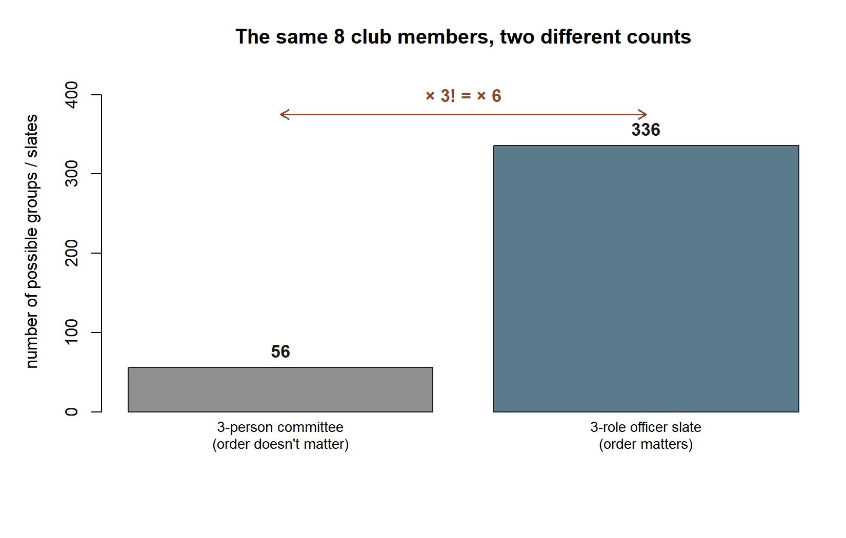
The ratio between the two answers is no coincidence: \(336 = 56 \times 3! = 56\times 6\). Each unordered committee of three can be assigned to the three roles in \(3!=6\) ways, which is precisely the \(k!\) factor that separates a permutation from a combination. Seeing that \(336 = 56\times 6\) in a concrete case is the single clearest way to remember why \(\binom{n}{k}=\frac{1}{k!}\cdot\frac{n!}{(n-k)!}\).

Putting the two counts side by side, from the same \(8\) members, makes the \(\times 6\) gap between them concrete rather than abstract.

Figure 4: One club, two very different counts (synthetic). The \(3\)-person committee count (\(56\)) and the \(3\)-role officer-slate count (\(336\)), both drawn from the same \(8\) club members. The officer count is exactly \(6=3!\) times the committee count.

What the figure shows (non-visual equivalent). Two bars from the identical \(8\)-member pool: \(56\) committees (order-free) versus \(336\) officer slates (order matters), with \(336=56\times 6\). Synthetic instructional example; numbers are illustrative.

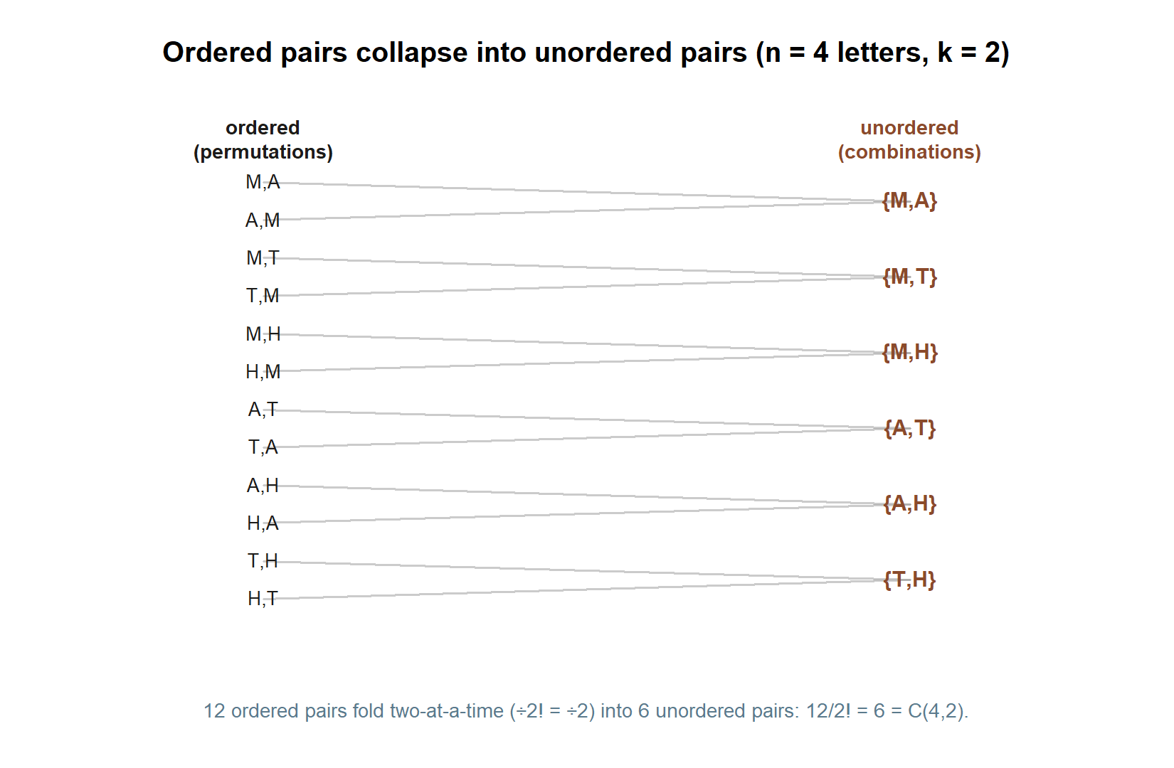
The same split appears in the classic “arrange the letters” question. Arranging the \(4\) distinct letters of the word MATH in a row is an ordered, fill-every-slot problem, so there are \(4!=24\) arrangements; but if we only asked which two of the four letters to keep (no order), that would be \(\binom{4}{2}=6\). Order in the row makes it a factorial; ignoring order makes it a combination.

The same MATH letters make the folding relationship between the two counts visible directly: list every ordered pair of two letters, then watch pairs fold together whenever they name the same unordered set.

Figure 5: Ordered pairs folding into unordered pairs (synthetic). All \(4\times3=12\) ordered pairs of two distinct letters from MATH, each connected to the one unordered pair \(\{\cdot,\cdot\}\) it belongs to. Every unordered pair receives exactly \(2=2!\) ordered pairs, so \(12/2!=6=\binom{4}{2}\).

What the figure shows (non-visual equivalent). The \(12\) ordered pairs (MA, AM, MT, TM, …) fold two at a time onto the \(6\) unordered pairs ({M,A}, {M,T}, …) — MA and AM both land on {M,A}, and so on. This is the \(k!=2!=2\) factor in \(\binom{n}{k}=\frac{1}{k!}\cdot\frac{n!}{(n-k)!}\) made visible, the same relationship the committee/officer figure above showed with \(k!=6\). Synthetic instructional example; numbers are illustrative.

A common mistake

The most common — and most expensive — counting error is using a permutation where a combination belongs, or vice versa, because the “order matters?” question went unasked.

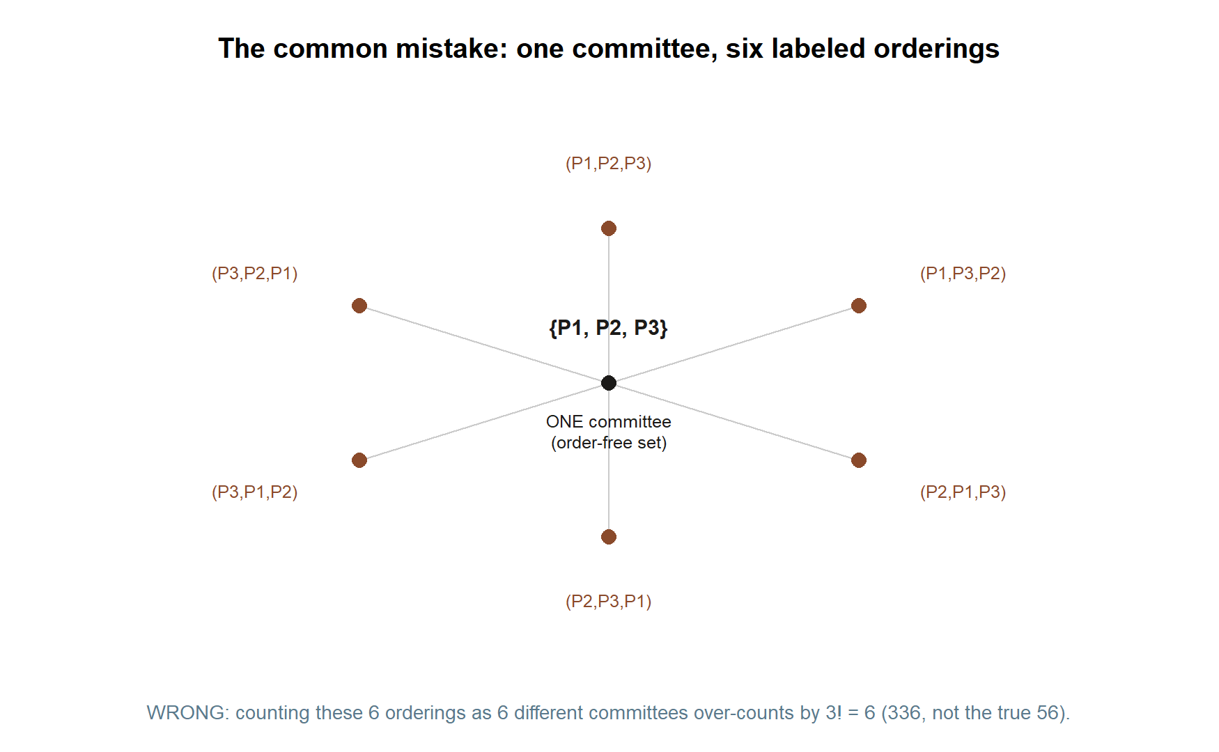
Watch what happens if we had answered the committee question (Version A) with a permutation. We would have reported \(\frac{8!}{5!}=336\) committees instead of \(56\), over-counting by a factor of \(3!=6\), because we would have treated the same three people listed in a different order as six different committees. They are not different — a committee has no internal order — so \(336\) is simply wrong for that question. The over-count flows straight into the probability: a “\(1/336\)” answer would be off by a factor of six.

Drawing the six orderings of a single, specific committee side by side is the clearest way to see the mistake happening.

Figure 6: The over-count, drawn (synthetic). One specific committee, \(\{P1,P2,P3\}\), and its \(3!=6\) orderings. Treating the six orderings as six different committees is exactly the error described above.

What the figure shows (non-visual equivalent). One committee, \(\{P1,P2,P3\}\), sits at the center; the six labeled orderings around it — \((P1,P2,P3)\), \((P1,P3,P2)\), and so on — are all the same committee. Counting each ordering as a separate committee is precisely how \(56\) becomes the wrong answer \(336\). Synthetic instructional example; numbers are illustrative.

The discipline that prevents this is to ask one question before reaching for a formula: if I shuffle the selection, is it a different outcome? Officers with titles — yes, shuffle changes who is president — so count ordered. A title-free committee — no, shuffling the names changes nothing — so count unordered. A second guard is the relationship \(\binom{n}{k}=\frac{1}{k!}\cdot\frac{n!}{(n-k)!}\): a permutation is always \(k!\) times the matching combination, so if your two answers do not differ by exactly \(k!\), you have mixed up which is which.

Low-stakes self-checks (ungraded)

These are for your own practice — ungraded, no submission, just a way to test your understanding.

1. A lunch special lets you pick one of \(3\) soups and one of \(4\) sandwiches. Use the multiplication principle to count the possible lunches. (Then: does order of choosing matter here?)
2. Compute \(\binom{6}{2}\) and \(\frac{6!}{(6-2)!}\) by hand. Confirm that the permutation is exactly \(2!=2\) times the combination, and explain in one sentence why.
3. On the ten-question true/false quiz, write down \(P(\text{exactly }10\text{ correct})\) and \(P(\text{exactly }0\text{ correct})\) as fractions over \(1024\). Why are they equal?
4. A book club of \(7\) readers picks a \(4\)-person discussion panel with no roles. How many panels are possible? Then suppose the panel needs an ordered reading order instead — how many orderings? Check that the second answer is \(4!\) times the first.
5. Rearrange the letters of the (distinct-letter) word PRIME: how many distinct arrangements are there? Which counting tool did you use, and why?

A self-check: try to state, in one sentence each, which tool (multiplication principle, permutation, or combination) each problem needs and why, before you compute. Naming the tool is the skill; the arithmetic follows.

Reading and source pointer

The primary reading for this week is Grinstead & Snell, Introduction to Probability, Chapter 3 (Combinatorics) — the multiplication principle, permutations, factorials, and combinations, including the “choose” notation and the binomial-coefficient identities we used. It is free online: https://www.dartmouth.edu/~chance/teaching_aids/books_articles/probability_book/book.html.

There is no MIT 18.05 pointer this week — the secondary source is genuinely used in the conditional- probability, Bayes, standard-model, simulation, and review weeks, but Chapter 3’s counting material is fully served by the Grinstead & Snell reading above.

These notes are the course’s own synthesis, grounded in but not copied from the sources.

Public vs. graded

These notes, the examples, and the practice here are public and ungraded — study material only. No graded prompts, answer keys, rubrics, point values, or due dates appear on this site. Graded checkpoints, quizzes, homework, labs, the midterm, the project, and the final live in Blackboard (the LMS), which is authoritative for due dates, submissions, and grades. If this page and Blackboard ever disagree, follow Blackboard.

Looking ahead

Counting is the launch pad for the discrete-distribution arc. In Week 7 we attach a number to each outcome — a random variable — and the by-score counts \(\binom{10}{k}\) you built here become the probability mass function of the guessing student’s score. In Week 8 we summarize that pmf with an expectation (\(E[X]=5\)) and a variance (\(\operatorname{Var}(X)=2.5\)), and in Week 9 we recognize the whole pattern as the Binomial\((10,0.5)\) distribution and name it. Every one of those steps reuses the combination \(\binom{10}{k}\) and the total \(2^{10}=1024\) from this week — so the counting you practiced now is the scaffolding for the next three.

See also

• Notation glossary — the binding symbols for \(\binom{n}{k}\), factorials, \(P(\cdot)\), and the equally-likely model.
• Distribution reference — where the binomial coefficient reappears as the heart of the Binomial pmf in the coming weeks.
• Week 7 — Discrete random variables — the immediate next step, where these counts become a pmf.
• Course syllabus — the official schedule, policies, and authoritative course information.