set.seed(35003)
# Synthetic illustration only; the named model arrives in Week 11.
# Mean wait near 15 minutes -> rate = 1/15 per minute.
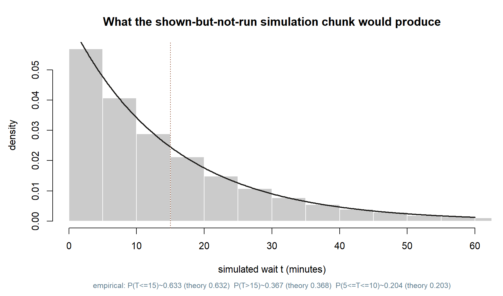
t <- rexp(100000, rate = 1/15)            # many simulated waits (minutes)

mean(t <= 15)                              # ~ P(T <= 15) ~ 0.632  (area to the left of 15)
mean(t >  15)                              # ~ P(T > 15)  ~ 0.368  (right-tail area)
mean(t >= 5 & t <= 10)                     # ~ P(5 <= T <= 10) ~ 0.203 (middle strip)
mean(t == 7) # ~ 0: an exact value has probability 0Week 10 — Continuous random variables
Densities, cdfs, and probability as area
Mathematical goal
By the end of this week you should be able to read a continuous random variable through three connected objects and move between them without confusion:
- the density \(f(x)\), a height function that is not a probability;
- probability as area, \(P(a\le X\le b)=\int_a^b f(x)\,dx\); and
- the cumulative distribution function (cdf) \(F(x)=P(X\le x)=\int_{-\infty}^{x} f(t)\,dt\), whose slope recovers the density, \(f(x)=F'(x)\).
The single most important habit to build is treating \(f(x)\) as a rate of probability per unit of \(x\), so that you only ever turn it into an actual probability by integrating — by accumulating area across an interval. This is the continuous mirror of the discrete pmf \(p(x)\) you met in Weeks 7–9, and getting the mirror right is what lets the named models in Week 11 (the exponential and the normal) make sense.
The week question
So far every random variable we have studied has been discrete: the quiz score \(X\) took whole-number values \(0,1,\dots,10\), and we could list a probability \(p(x)=P(X=x)\) for each one. But many quantities are not like that. Consider Maya’s commute again, and this time start a stopwatch the instant she reaches the stop: let
\[ T = \text{the time she waits until the next shuttle arrives.} \]
\(T\) is a continuous quantity — it could be \(3\) minutes, or \(3.4\), or \(3.41719\ldots\); between any two possible waits there is always another. The week’s question is: how do we put probabilities on a quantity that can take uncountably many values, where listing \(P(T=x)\) for every single \(x\) is hopeless? The answer reorganizes everything around area under a curve rather than a sum over a list, and it forces one surprising fact: the probability that \(T\) equals any exact value is zero, even though \(T\) certainly takes some value.
Notation
| Symbol | Meaning |
|---|---|
| \(X,\ T\) | a continuous random variable (here \(T\) = wait until the next shuttle) |
| \(f(x)\), \(f_X(x)\) | the probability density function — a height, not a probability; may exceed \(1\) |
| \(F(x)\), \(F_X(x)\) | the cumulative distribution function, \(F(x)=P(X\le x)\) |
| \(\displaystyle\int_a^b f(x)\,dx\) | the area under \(f\) between \(a\) and \(b\) — this is a probability |
| \(f(x)=F'(x)\) | density is the derivative (slope) of the cdf |
| \(U\sim\text{Uniform}(0,1)\) | the continuous uniform on \([0,1]\) (the spinner) |
| \(\lambda\) | a rate (used loosely this week; formalized for the exponential in Week 11) |
Two reminders carried forward from the notation glossary: “\(\le\)” versus “\(<\)” will turn out not to matter for a continuous variable (a single point carries no probability), and densities are written with \(f\) to keep them visibly distinct from the discrete mass function \(p\).
Conceptual setup
From a histogram of mass to a curve of density
Recall how a discrete variable assigns probability: each value \(x\) gets a lump \(p(x)=P(X=x)\). Picture those lumps as the bars of a histogram, each bar’s area equal to its probability. Now measure the wait \(T\) more and more finely — to the minute, then the second. The bars get narrower, and to keep each bar’s area equal to the probability of that narrow slice, the bars’ heights must change. In the limit the tops of the bars trace a smooth curve: the density \(f(x)\). The rule that survives the limit is the one that matters — probability is still area, but area is now computed by integration instead of by adding up finitely many bars.
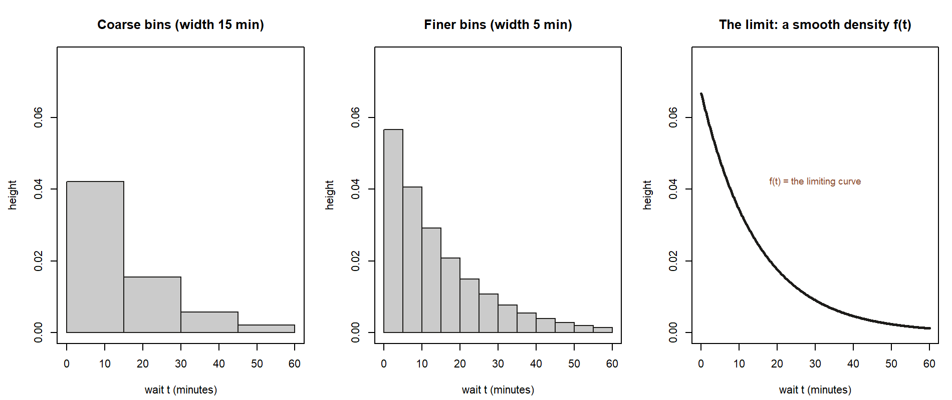
So a density must satisfy two conditions, exactly mirroring “\(p(x)\ge 0\) and \(\sum_x p(x)=1\)” from the discrete world:
\[ f(x)\ge 0 \quad\text{for all } x, \qquad\qquad \int_{-\infty}^{\infty} f(x)\,dx = 1 . \]
The first says the curve never dips below the axis (a negative probability rate would be meaningless). The second says the total area under the whole curve is \(1\) — all the probability is accounted for.
The density is a height, not a probability
Here is the convention this whole week is built to protect. \(f(x)\) is not \(P(X=x)\). For a continuous variable, \(P(X=x)=0\) for every single value \(x\), because a single point is an interval of width \(0\), and an area of zero width is zero:
\[ P(X=a)=\int_a^a f(x)\,dx = 0 . \]
That is not a paradox. It says only that no individual exact value is favored enough to carry positive probability on its own; the probability lives in intervals, in stretches of \(x\), never in points. A direct and useful consequence is that the endpoints do not matter:
\[ P(a\le X\le b)=P(a< X< b)=P(a\le X< b)=P(a<X\le b)=\int_a^b f(x)\,dx . \]
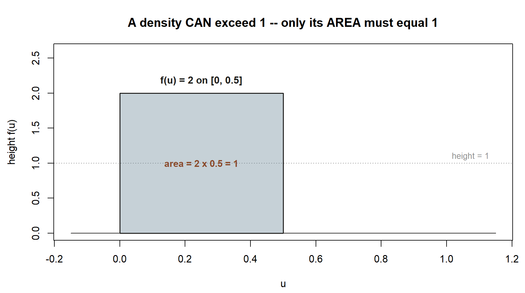
A second consequence catches almost everyone: \(f(x)\) can be larger than \(1\). A density is a probability per unit of \(x\), not a probability, so its height is unbounded — on a narrow \(x\)-axis the curve can rise well above \(1\) and still enclose total area \(1\). Only the area is a probability, always between \(0\) and \(1\).
The cdf accumulates the area
Integrating the density from the far left up to a moving cutoff \(x\) defines the cumulative distribution function:
\[ F(x)=P(X\le x)=\int_{-\infty}^{x} f(t)\,dt . \]
\(F\) answers “how much probability has piled up by the time we reach \(x\)?” It starts at \(0\) on the far left, climbs (never decreases, since \(f\ge 0\) adds only non-negative area), and levels off at \(1\) on the far right:
\[ \lim_{x\to-\infty}F(x)=0, \qquad \lim_{x\to\infty}F(x)=1, \qquad F \text{ is non-decreasing.} \]
The cdf and the density are two views of the same object, linked by the Fundamental Theorem of Calculus. Going forward, integrate the density to get accumulated probability; going backward, differentiate the cdf to recover the density:
\[ F(x)=\int_{-\infty}^{x} f(t)\,dt \qquad\Longleftrightarrow\qquad f(x)=F'(x) . \]
Interval probabilities then drop out of the cdf by subtraction, which is often the fastest route in practice:
\[ P(a\le X\le b)=\int_a^b f(x)\,dx = F(b)-F(a). \]
This is the continuous analogue of the discrete “add the relevant masses,” with \(F(b)-F(a)\) playing the role of “the running total at \(b\) minus the running total at \(a\).”
Worked example
We work the recurring slice symbolically first, then put numbers on it. (All data are synthetic; seed 35003 set. The numbers here are illustrative — the named distribution for \(T\) is introduced next week.)
Worked example — the shuttle wait \(T\) as area under a density (recurring slice)
Setup. Maya reaches the stop and waits time \(T\) for the next shuttle. Shuttles come at a steady average rate, and \(T\) is a positive continuous waiting time: \(T\ge 0\). Suppose its behavior is captured by a density \(f(t)\) that is zero for \(t<0\) (you cannot wait a negative time), is largest near \(t=0\) (short waits concentrate there), and tapers off as \(t\) grows (long waits get rarer). We do not need the formula yet — Week 11 will name it the exponential, \(f(t)=\lambda e^{-\lambda t}\). This week we only read probabilities off the curve as areas.
Symbolic form. Whatever the exact \(f\), the rules from the setup apply unchanged:
\[ P(a\le T\le b)=\int_a^b f(t)\,dt, \qquad F(t)=P(T\le t)=\int_0^{t} f(s)\,ds, \qquad f(t)=F'(t). \]
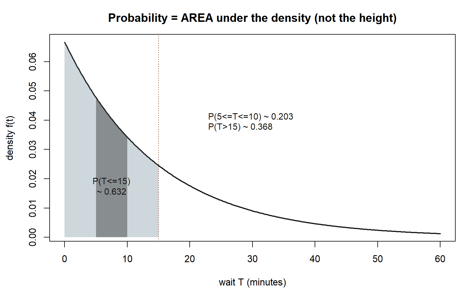
The probability that Maya waits between \(a\) and \(b\) minutes is the area under \(f\) over the strip \([a,b]\). The probability she waits at most \(t\) minutes is the area from the start out to \(t\) — exactly \(F(t)\). And the chance she waits more than \(t\) minutes is the complement, the leftover area to the right:
\[ P(T>t)=1-P(T\le t)=1-F(t). \]
Reading off three quantities. Suppose, for this illustration, that the cdf has the shape \(F(t)=1-e^{-t/15}\) for \(t\ge 0\), with \(t\) in minutes (this is the running-total curve that goes with the “average wait near 15 minutes” picture; Week 11 derives it). Then probabilities are just differences of \(F\):
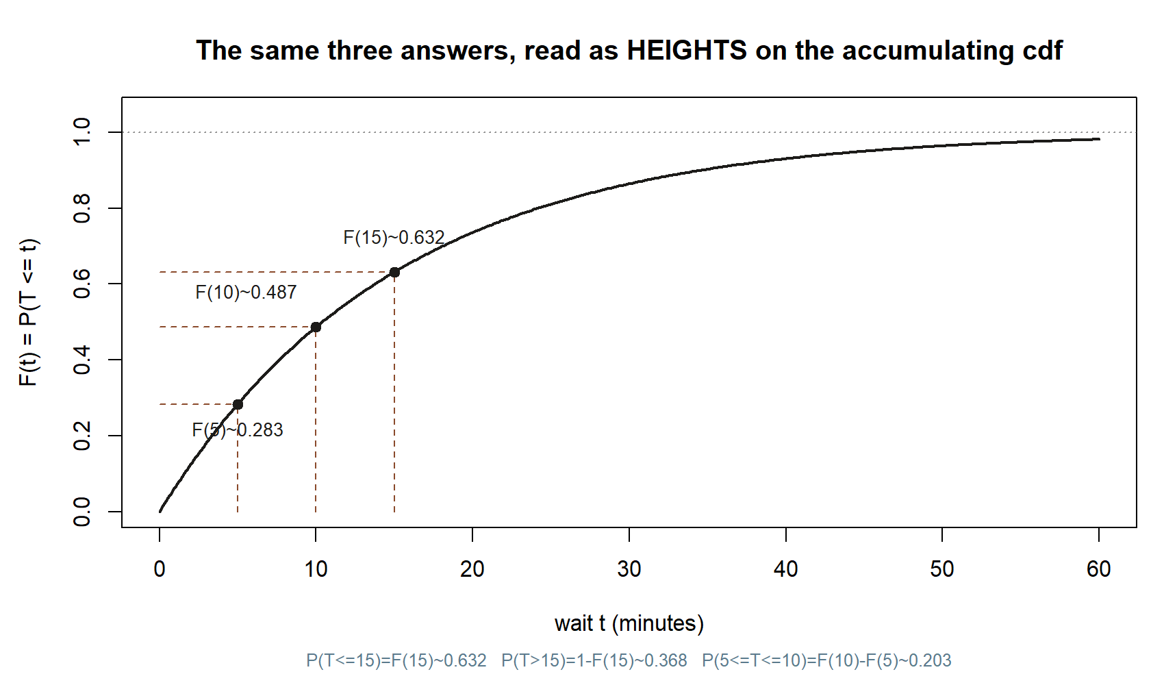
- Wait at most 15 minutes. The accumulated area out to \(t=15\) is \[ P(T\le 15)=F(15)=1-e^{-15/15}=1-e^{-1}\approx 0.632 . \]
- Wait more than 15 minutes. The complementary (right-tail) area is \[ P(T>15)=1-F(15)=e^{-1}\approx 0.368 . \]
- Wait between 5 and 10 minutes. The strip of area between \(5\) and \(10\) is \[ P(5\le T\le 10)=F(10)-F(5)=\bigl(1-e^{-10/15}\bigr)-\bigl(1-e^{-5/15}\bigr) = e^{-1/3}-e^{-2/3}\approx 0.7165-0.5134 \approx 0.203 . \]
Interpretation. Each answer is a region of the curve: a left chunk for “at most,” a right tail for “more than,” a middle strip for “between.” Asking for an exact wait — “\(P(T=7)\)” — gives a strip of zero width, hence probability \(0\): Maya will wait some specific time, but no single exact time carries positive probability by itself. We re-meet \(F(15)=1-e^{-1}\approx 0.632\) next week as the headline exponential result — keep the number in view.
The same three answers can also be read off the cdf directly, as heights rather than areas — a second representation of the identical facts:
If we wanted to see this rather than integrate by hand, the shown-as-teaching simulation below draws many synthetic waits and reports the fraction that land in each region; the fractions track the areas above. Code is shown for teaching and is not run in this build.
This chunk is a run-it-yourself teaching activity, not executed evidence on its own — the figure below is what running it produces (same seed, same sample size, same rate), shown here so the connection between code and picture does not have to be taken on faith:
Worked example — a Uniform(0,1) spinner, area as a rectangle (transfer)
Setup. Spin a perfectly balanced pointer that stops at an angle, and rescale the reading so it lands somewhere in \([0,1]\) with no part of the dial favored. Call the result \(U\), so \(U\sim\text{Uniform}(0,1)\). “No part favored” means the density is flat across \([0,1]\) and zero outside it. (Synthetic; seed 35003 set.)
Symbolic form. A flat density on \([0,1]\) must have constant height \(c\), and total area \(1\) forces \(c\cdot(1-0)=1\), so \(c=1\):
\[ f(u)= \begin{cases} 1, & 0\le u\le 1,\\[2pt] 0, & \text{otherwise.} \end{cases} \]
Here the density’s height is exactly \(1\) — a clean reminder that the height carries no probability by itself; only area does. Probabilities are areas of rectangles under this flat top:
\[ P(a\le U\le b)=\int_a^b 1\,du = b-a, \qquad 0\le a\le b\le 1 . \]
The cdf is the running area from the left edge, a straight ramp from \(0\) to \(1\):
\[ F(u)=\int_0^{u} 1\,ds = u,\qquad 0\le u\le 1 . \]
Numeric form. The chance the spinner lands between \(0.2\) and \(0.5\) is the area of the rectangle of width \(0.5-0.2\) and height \(1\):
\[ P(0.2\le U\le 0.5)=\int_{0.2}^{0.5} 1\,du = F(0.5)-F(0.2)=0.5-0.2 = 0.3 . \]
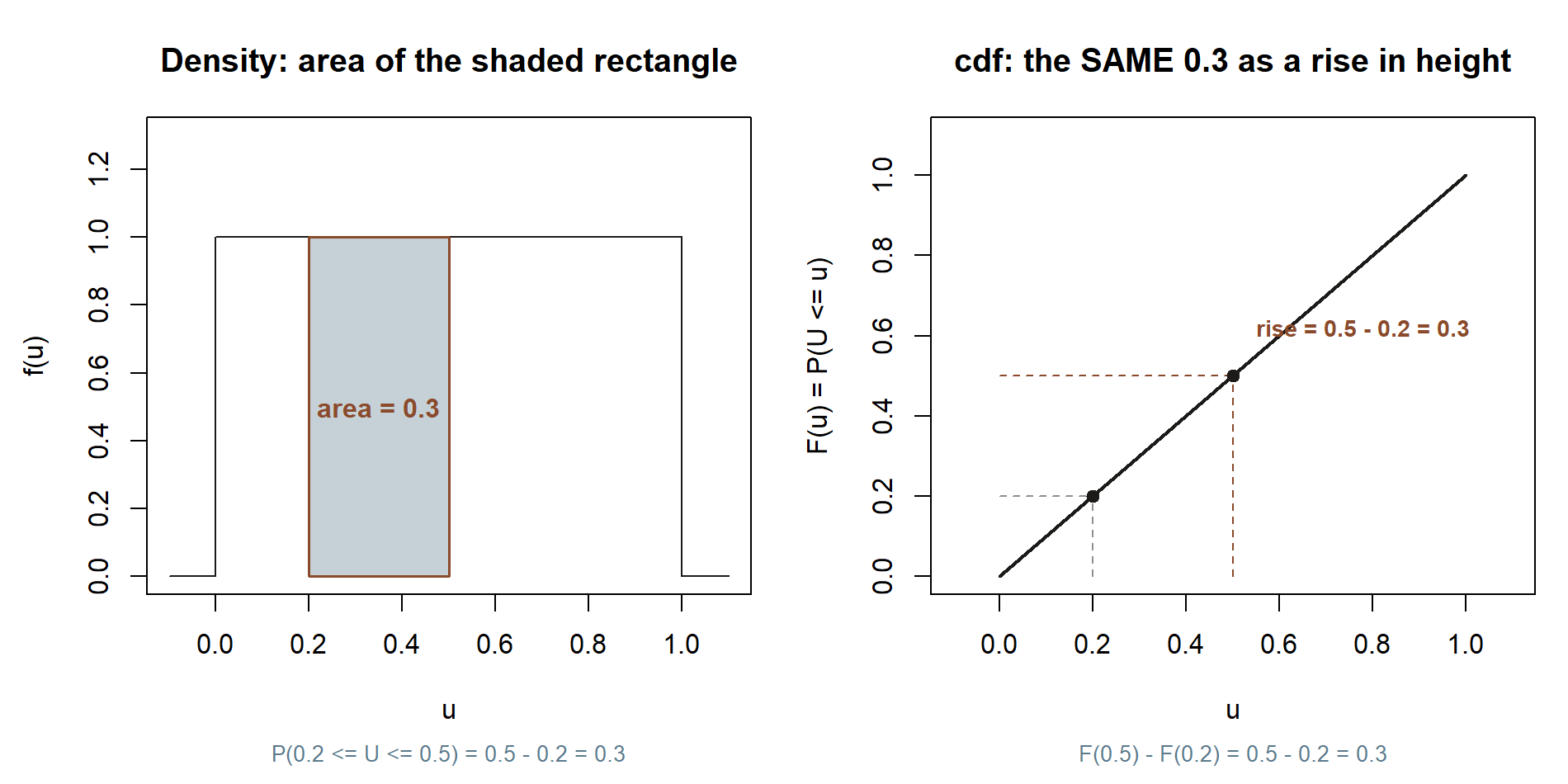
Interpretation. A width-\(0.3\) slice of a height-\(1\) flat density encloses area \(0.3\), so the spinner lands in \([0.2,0.5]\) about \(30\%\) of the time. Endpoints are irrelevant — \(P(0.2<U<0.5)\) is the same \(0.3\), since each endpoint is a width-\(0\) strip with zero area. This is the continuous idea at its simplest: probability is the area of a region under the density, and a rectangle is the easiest region to measure.
A convention warning
The convention this week exists to protect — and the one the notation glossary flags explicitly — is this:
A density value \(f(x)\) is not a probability. It is a probability rate per unit of \(x\). You convert it into a probability only by integrating it over an interval (taking an area). Consequences you must keep straight:
- \(f(x)\) can be greater than \(1\) and that is fine; only an area must lie in \([0,1]\).
- \(P(X=x)=0\) for every exact \(x\) — a continuous variable puts no probability on points.
- Because points carry no probability, \(\le\) and \(<\) are interchangeable: \(P(a\le X\le b)=P(a<X<b)\).
- To get a number, integrate \(f\) (or, equivalently, subtract cdf values \(F(b)-F(a)\)). Reading a density height as if it were the probability is the classic error this course guards against.
Mirror-image caution in the other direction: do not sum a density the way you summed a pmf. There is no “\(\sum_x f(x)=1\)” for a continuous variable — the matching statement is “\(\int f(x)\,dx=1\),” an area, not a sum. The discrete machinery of Weeks 7–9 and the continuous machinery of this week are analogues, not the same operations; keep “sum the masses” and “integrate the density” in separate mental drawers.
Practice (ungraded)
These are for your own checking — ungraded, no submission. Work them symbolically first, then put numbers in.
- Density basics. A continuous variable has density \(f\) on the whole line. State in your own words why each is true: (a) \(f(x)\ge 0\) everywhere; (b) the total area under \(f\) is \(1\); (c) \(f(x)\) may exceed \(1\);
- \(P(X=3)=0\).
- Uniform rectangle. For the spinner \(U\sim\text{Uniform}(0,1)\), find \(P(U\le 0.4)\), \(P(U>0.75)\), and \(P(0.1\le U\le 0.6)\) by drawing the rectangle and computing its area. Confirm each equals the matching difference of \(F(u)=u\).
- Wider uniform. Suppose a different spinner gives \(V\sim\text{Uniform}(0,2)\). What constant height must its density have so the total area is \(1\)? Is that height above or below \(1\)? Find \(P(0.5\le V\le 1.5)\). (Self-check: height \(=\tfrac12\); the answer is \(\tfrac12\).)
- Shuttle wait as area. Using the illustrative cdf \(F(t)=1-e^{-t/15}\) for the wait \(T\) (minutes), set up — and then evaluate — (a) \(P(T\le 10)\), (b) \(P(T>20)\), (c) \(P(10\le T\le 20)\). Which one is a left chunk, which a right tail, which a middle strip?
- Density from a cdf. If a cdf is the ramp \(F(x)=x\) on \([0,1]\), recover the density by differentiating, \(f(x)=F'(x)\). What familiar density do you get, and what is its height?
- Endpoints don’t matter. Argue, using \(P(X=a)=0\), why \(P(a\le X\le b)\) and \(P(a<X<b)\) are equal for any continuous \(X\). Where does this fail for a discrete variable, and why?
Reading and source pointer
- Grinstead & Snell, Introduction to Probability, Chapter 2 — Continuous Probability Densities — grounds the density/area/cdf machinery and the “probability as area” picture at the right first-course depth. Free online text.
(No MIT 18.05 pointer this week; the standard continuous models — exponential and normal — are pointed to in Week 11.)
These notes are the course’s own synthesis, grounded in but not copied from the sources.
Public vs. graded
These notes, the examples, and the practice here are public and ungraded — study material only. No graded prompts, answer keys, rubrics, point values, or due dates appear on this site. Graded checkpoints, quizzes, homework, labs, the midterm, the project, and the final live in Blackboard (the LMS), which is authoritative for due dates, submissions, and grades. If this page and Blackboard ever disagree, follow Blackboard.
Looking ahead
This week built the general continuous machinery — density, area, cdf — without committing to a particular curve. Week 11 names two specific densities and puts them to work: the exponential \(f(t)=\lambda e^{-\lambda t}\) for the shuttle wait \(T\) (with rate \(\lambda=4\) per hour, so a mean wait of \(15\) minutes and \(P(T\le 15\text{ min})=1-e^{-1}\approx 0.632\) — the very number we previewed above), and the normal \(\mathcal N(\mu,\sigma)\) for Maya’s commute time. With named models in hand, “probability as area” becomes “look up or compute a specific area,” and the cdf becomes a tool you reach for constantly.
See also
- Week 9 — Common discrete models — the discrete pmf side this week mirrors (Poisson counts of shuttle arrivals).
- Week 11 — Common continuous models — names the exponential and normal densities and revisits the shuttle wait \(T\).
- Notation glossary — the binding meanings of \(f(x)\), \(F(x)\), and the “density is not a probability” convention.
- Distribution reference — the continuous models (uniform, exponential, normal) and their parameterizations.
- Course syllabus — schedule, policies, and how the public site relates to Blackboard.