set.seed(35003)
n_weeks <- 100000
# each week: 5 independent mornings, each late with probability 0.19
late_counts <- rbinom(n_weeks, size = 5, prob = 0.19)
mean(late_counts == 0)   # close to 0.349
mean(late_counts == 1)   # close to 0.409
mean(late_counts >= 2)   # close to 0.242
mean(late_counts) # close to the mean 5 * 0.19 = 0.95Week 14 — Probability modeling project
Building, simulating, and defending a small probability model
The week question
Almost everything so far has handed you the model. The problem said “a fair coin,” or “shuttles arrive Poisson at rate four per hour,” or “commute time is Normal with mean 22 and standard deviation 5,” and your job was to compute from there. That is the right way to learn the machinery, but it hides the hardest and most useful step in real probability work: nobody hands you the model. You start with a vague question about an uncertain situation, and you have to decide what random variable to use, what distribution to put on it, and what assumptions you are quietly buying when you do.
So this week’s question is a working one rather than a new piece of theory: how do you take a fuzzy real-world question, turn it into a small probability model, check that model against a simulation, and then honestly say what it does and does not capture? This is a workshop week. The math is lighter than usual and almost all of it is machinery you already own — Bernoulli trials, the binomial, expectation, simulation. What is new is the loop that ties them together into a defensible little argument, and the discipline of saying out loud where your model could be wrong.
Why this matters
A probability model is a deliberate simplification of the world, built to answer one question. Its value is never that it is “true” — it is always an approximation — but that it is useful and honest: it gives you a number you can act on, together with a clear statement of the assumptions that number rests on. The whole craft is choosing assumptions that are simple enough to compute with and faithful enough to trust.
That craft is exactly what this week practices, because it is the step that does not show up in a final answer. A wrong arithmetic step gets caught when the numbers look strange. A wrong model produces numbers that look perfectly reasonable and are quietly meaningless — you can compute \(P(L \ge 2)\) to four decimals from a binomial that never should have been a binomial. The defense against that is not more algebra; it is the habit of stating assumptions before you compute and stress-testing them after.
There is a second payoff. When you build the model and simulate it, you get two independent routes to the same answer. If the theoretical probability and the simulated frequency agree, your confidence in both goes up; if they disagree, you have found a bug — in the formula, the code, or your understanding of the model — before it costs you anything. Maya’s commuter world gives us a small, concrete question to run the whole loop on, and then we sketch a second model in a fresh setting so you can see that the loop, not the example, is the transferable thing.
Learning goals
By the end of this week you should be able to:
- Take an informal question about an uncertain situation and restate it as a precise probability question about a named random variable.
- List the modeling assumptions a chosen distribution commits you to, and name at least one assumption that is most likely to fail.
- Build a small model from familiar pieces (Bernoulli trials, a binomial count, an expectation) and compute the quantity of interest symbolically first, then numerically.
- Simulate the same model in base R and compare the simulated frequency against the theoretical value as a check on both.
- Communicate a conclusion in plain language together with its limits — what the number means, and where the model could mislead.
Core vocabulary
- Model — a deliberately simplified probabilistic description of a situation, chosen to answer one question. Always an approximation, judged by usefulness and honesty, not truth.
- Modeling assumption — a condition you adopt so the math is tractable (for example, that trials are independent and identically distributed). Every distribution name carries a bundle of these.
- The modeling loop — choose a question → state assumptions → build the model → simulate → compare simulated vs theoretical → communicate the conclusion and its limits. The spine of this week.
- Theoretical value — the probability or expectation computed exactly from the model’s formula.
- Simulated estimate — the same quantity approximated by generating many random draws and taking a frequency or average; it should land near the theoretical value, with sampling wobble that shrinks as the number of draws grows (this is the law of large numbers from Week 13 doing its job).
- Sensitivity — how much the answer moves when you nudge an assumption or a parameter; a model whose conclusion flips under a small, plausible change deserves a caveat.
Concept development
The modeling loop, step by step
Treat a model as a short argument with six moves, taken in order. Skipping a step is how silent errors get in, so it is worth naming each one.
- Choose the question. Pin down exactly what you want a probability or an expectation of. “Will Maya be late a lot?” is not yet a probability question; “what is the chance she is late on at least two of five weekday mornings?” is.
- State the assumptions. Decide what random variable describes the situation and what distribution to put on it — and say, in words, what that choice commits you to. This is the step that does the real work and the one most often skipped.
- Build the model. Write the random variable, its distribution, and the formula for the target quantity. Keep it symbolic at first so the structure is visible before any number goes in.
- Simulate. Generate many draws from the model and estimate the same quantity as a frequency or an average. This is an independent check that does not rely on your formula being right.
- Compare. Put the theoretical value next to the simulated estimate. Agreement is reassurance; a gap is a flag to debug the formula, the code, or the assumptions.
- Communicate. State the conclusion in a sentence a non-specialist could act on, and immediately state its limits — which assumption is shakiest and which way the answer would move if it failed.
Before the words, here is the same six moves as a picture — the loop shape both worked examples below walk:
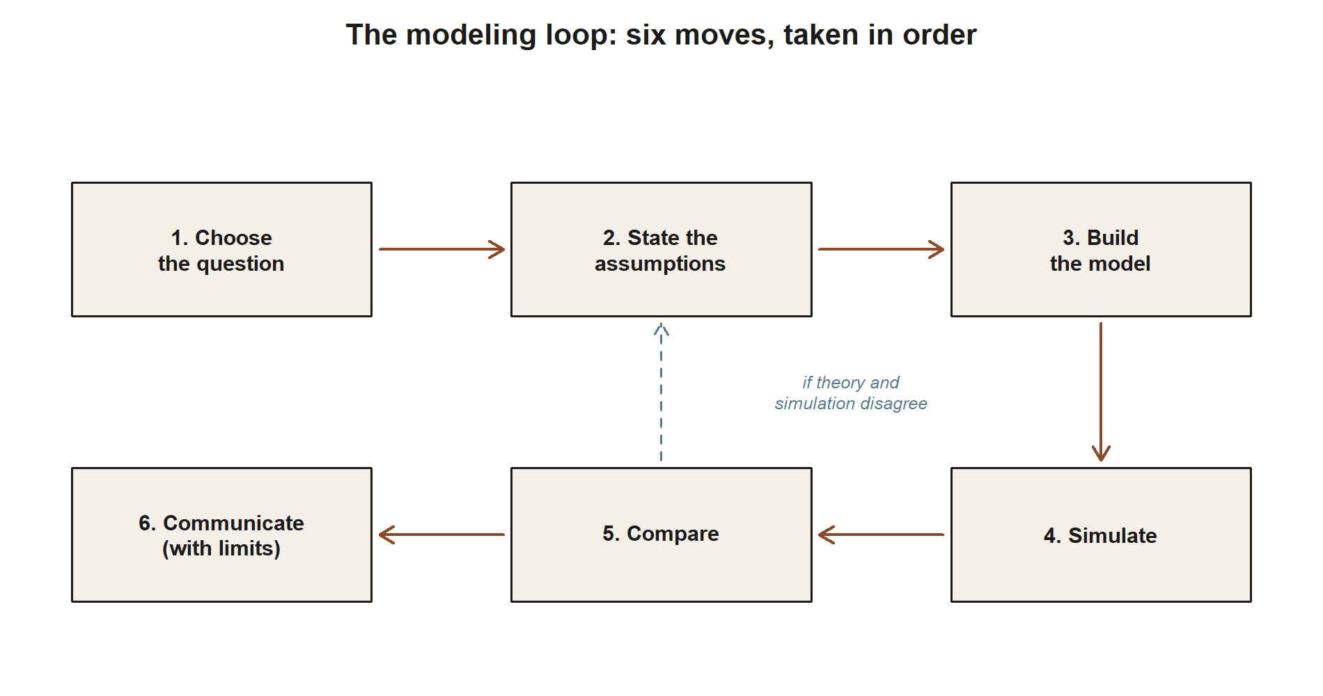
The loop is deliberately humble. Steps 2 and 6 are about honesty, not computation, and they are what separate a usable model from a number with no warranty.
Where independence is the load-bearing assumption
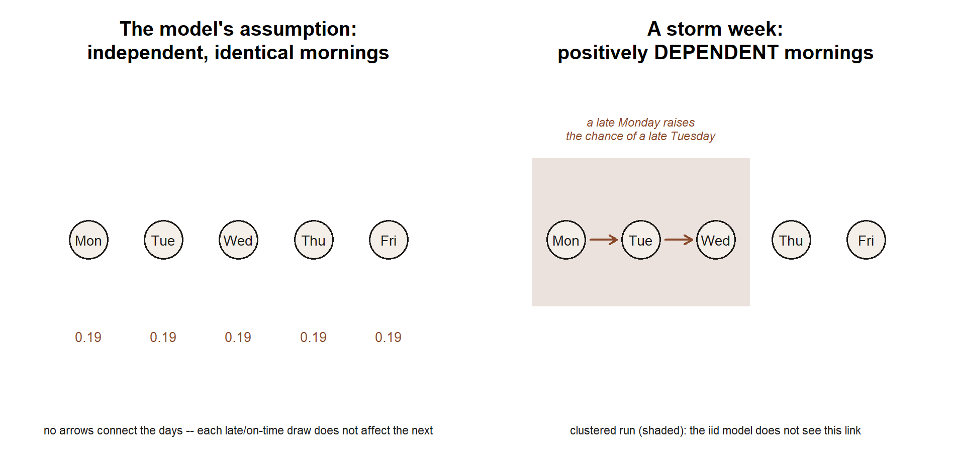
Most small first-course models lean hardest on independence and on identical distribution across trials — the “iid” assumption. It is load-bearing because it is exactly what lets you multiply probabilities and stack Bernoulli trials into a binomial. It is also the assumption most likely to be only approximately true.
In Maya’s world, “each weekday morning is an independent lateness trial with the same probability” is a clean modeling choice, but you can already feel where it might bend. A snowstorm that parks itself over the city for three days makes consecutive mornings positively dependent — a late Monday raises the chance of a late Tuesday — and it makes the per-day probability non-constant across that stretch. Neither failure makes the model useless; both make it a place to add a caveat. The discipline is to notice the assumption while you are choosing it, not after a reviewer points it out.
Why simulate something you can already compute
It can feel redundant to simulate a probability you can get exactly from a formula. The point is precisely that you can check it, and the checking is the training. When the formula is simple, simulation confirms you applied it correctly and that your mental model of the random process matches the code. When you later meet a model whose probability has no tidy closed form — and you will — simulation will be the only route, and you will trust it because you watched it agree with the formula in cases you could verify by hand. A simulation that disagrees with a correct formula is just as valuable: it has caught a real mistake cheaply.
Worked examples
All numbers below are synthetic; seed 35003 is set for any simulation. The first example runs the full modeling loop on Maya’s commuter world; the second sketches a fresh model so you can see the loop transfer.
Worked example — “at least two late days in a five-day week” (recurring slice)
Step 1 — the question. Maya rides the campus shuttle on five weekday mornings. We want the probability that the shuttle is late on at least two of those five mornings. Write \(L\) for the number of late mornings in the week; the target is \(P(L \ge 2)\).
Step 2 — the assumptions. From the recurring shuttle thread, a single morning is late with probability \(0.19\). To build a weekly model we assume each morning is its own lateness trial, that the trials are independent, and that the per-morning late probability is the same \(0.19\) every day. That is the iid Bernoulli assumption, and it is exactly the thing to flag later: weather and schedule effects can link consecutive mornings, so independence is the assumption most at risk.
Step 3 — build the model. A single morning is a Bernoulli trial,
\[ D_i \sim \text{Bernoulli}(0.19), \qquad i = 1, \dots, 5, \]
with “late” coded as success. The count of late mornings is the sum of five independent identical Bernoulli trials, which is exactly the binomial setting from Week 9:
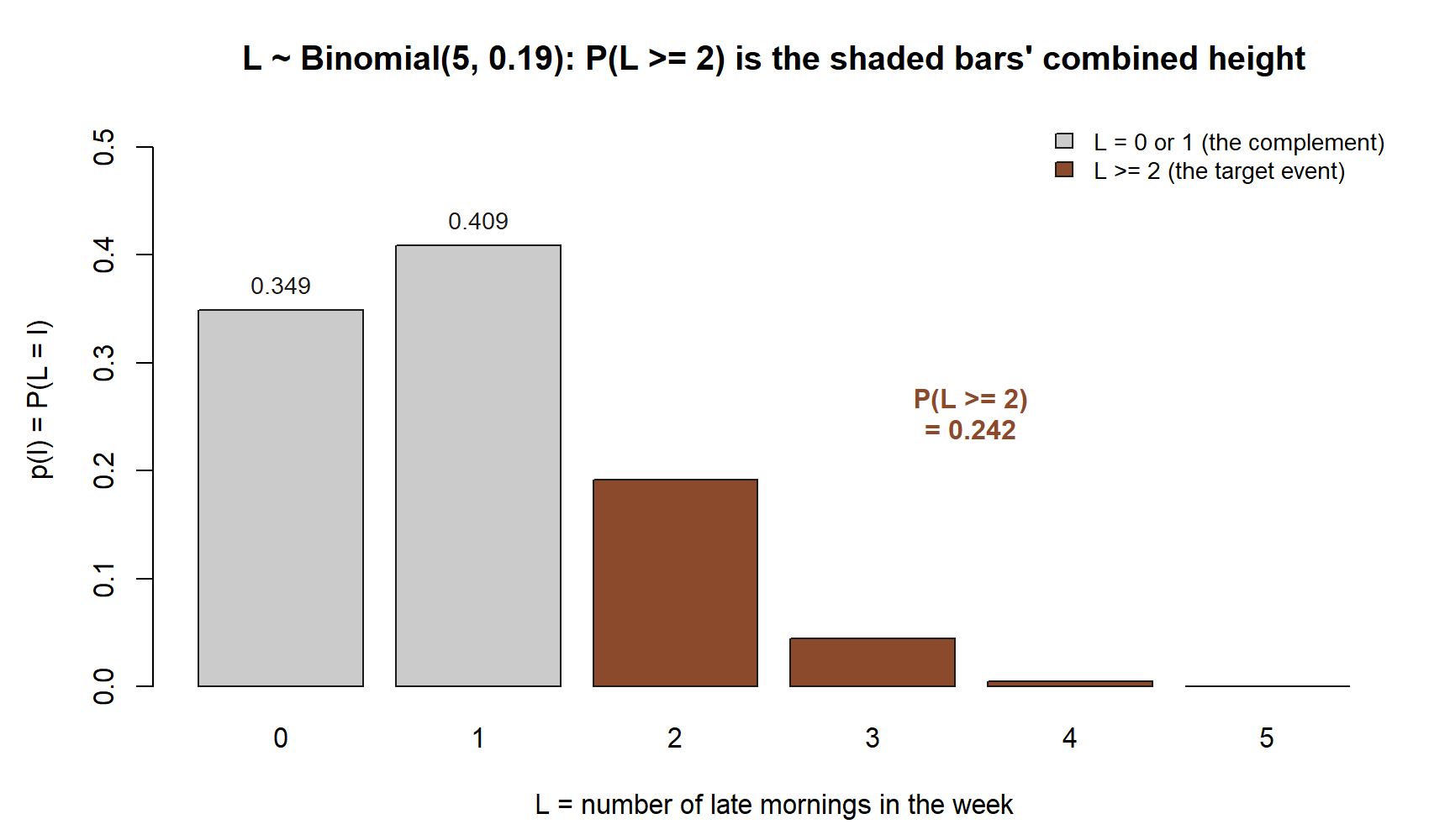
\[ L = \sum_{i=1}^{5} D_i \sim \text{Binomial}(5,\, 0.19), \qquad p(\ell) = \binom{5}{\ell}(0.19)^{\ell}(0.81)^{5-\ell}. \]
It is easier to find \(P(L \ge 2)\) through its complement than to add three terms, since “at least two” is everything except zero or one late morning:
\[ P(L \ge 2) = 1 - P(L = 0) - P(L = 1). \]
Numeric. The two small terms come straight from the pmf. A week with no late mornings needs all five to be on time:
\[ P(L = 0) = \binom{5}{0}(0.19)^{0}(0.81)^{5} = (0.81)^{5} \approx 0.349. \]
A week with exactly one late morning can place that one late day in any of five positions:
\[ P(L = 1) = \binom{5}{1}(0.19)^{1}(0.81)^{4} = 5\,(0.19)(0.81)^{4} \approx 0.409. \]
Subtracting both from one gives the target:
\[ P(L \ge 2) = 1 - 0.349 - 0.409 = 1 - 0.758 \approx 0.242. \]
So under the iid Bernoulli model, Maya faces a roughly 24% chance of two or more late mornings in a given five-day week — not rare at all. That already tells you something useful: “the shuttle is on time 81% of mornings” does not translate into “late weeks are unusual,” because the chances compound across five tries.
Step 4 — simulate. Generate many synthetic weeks, count late mornings in each, and estimate the same probability as a frequency (shown as teaching; not executed in this build):
Step 5 — compare. The three simulated frequencies should sit right on top of the theoretical \(0.349\), \(0.409\), and \(0.242\), with only small sampling wobble that shrinks as n_weeks grows — the law of large numbers from Week 13 at work. Agreement here means the formula and the code tell the same story; a gap would send you back to check whether the complement was set up correctly or whether rbinom was called with the right size and prob.
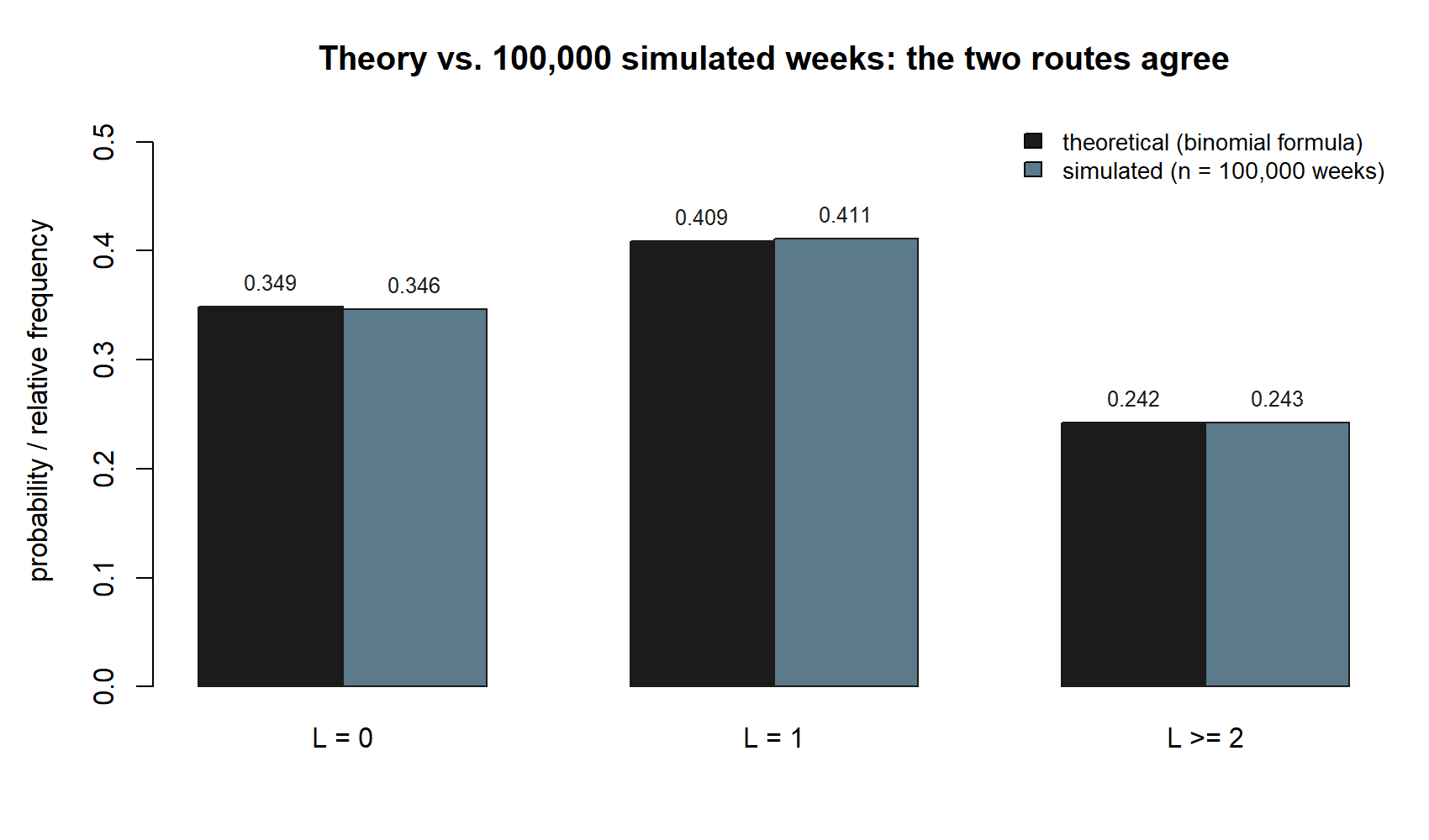
set.seed(35003)) — the bars are close to the same height in every pair.
Step 6 — communicate, with limits. The headline: under a model where each of five mornings is an independent, equally-likely 19%-late trial, the chance of two or more late mornings in a week is about 24%. The honest caveat lives in Step 2’s assumption. If mornings are positively dependent — a storm spanning several days, a recurring schedule conflict — late mornings would cluster, and the true chance of a multi-late week would be higher than the independence model says. The model gives a clean baseline; the caveat tells the reader which way reality is likely to bend it.
Worked example — expected buses caught in a week (transfer)
Now move the loop to a fresh question to show that the process, not the shuttle story, is what transfers. Suppose Maya also tries to catch a connecting city bus on each of the five weekday mornings, and on any given morning she makes it onto the bus with probability \(0.70\), independently across mornings. How many buses should she expect to catch in a week?
Run the same loop in miniature. The question is an expectation, \(E[B]\), where \(B\) is the number of buses caught in the week. The assumptions are again iid Bernoulli: five mornings, each a catch-or-miss trial with the same probability \(0.70\), independent of the others — and again, independence is the part to flag, since a single overslept morning could spill into the next. The model is therefore
\[ B \sim \text{Binomial}(5,\, 0.70), \qquad E[B] = np = 5\,(0.70) = 3.5. \]
So Maya should expect to catch about 3.5 buses in a typical five-day week.
![Bar chart of the Binomial(5, 0.70) pmf over 0 through 5 buses caught, rising to a peak at 4 and dropping at 5, with a dashed vertical line at 3.5 falling between the bars for 3 and 4, labeled E[B] = 3.5.](../assets/figures/wk14_buses_pmf_mean.png)
You could simulate it the same way — rbinom(n_weeks, size = 5, prob = 0.70) and take mean(...), which should land near \(3.5\) — and compare that average to the formula. The conclusion with limits: the iid model says about three and a half catches per week on average, but if missed mornings tend to come in runs (a rough week throwing off the whole routine), the count would be more variable than the independence model suggests even though its average stays near \(3.5\). Same six moves, brand-new setting. Synthetic; seed set.
A common mistake
The signature Week-14 mistake is computing past a broken assumption — reaching for the binomial because the surface story has “five mornings” in it, without pausing to ask whether those mornings are really independent and identically distributed. The binomial \(P(L \ge 2) \approx 0.242\) is exactly right given iid mornings; it can be badly wrong if a storm makes consecutive mornings dependent, and nothing in the arithmetic will warn you. The number will look just as clean either way.
A close cousin is reporting the point estimate with no caveat at all — handing over “about 24%” as if it were a fact about the world rather than a fact about a model. The whole reason Steps 2 and 6 bracket the computation is that the assumptions and the limits are part of the answer, not optional decoration. A third slip is mismatching the simulation to the model: simulating with the wrong prob, the wrong size, or the wrong event (counting >= 2 when you meant > 2), so the check silently “passes” against a model you did not intend. When the simulated frequency and the formula disagree, resist the urge to trust whichever one you like better; line up the model, the formula, and the code until you find which of the three is lying.
Low-stakes self-checks (ungraded)
These are for your own practice — nothing here is collected or graded.
- Restate each fuzzy question as a precise probability or expectation about a named random variable: (a) “does Maya usually have a smooth commute week?”; (b) “how often does she catch every bus?”; (c) “is a three-late-morning week common?” For each, name the random variable and the distribution you would use.
- For \(L \sim \text{Binomial}(5, 0.19)\), explain in one sentence why computing \(P(L \ge 2)\) through the complement \(1 - P(L=0) - P(L=1)\) is easier than summing \(p(2) + p(3) + p(4) + p(5)\), and confirm \(0.349 + 0.409 \approx 0.758\).
- State, in plain words, the two modeling assumptions the binomial model of late mornings commits you to, and describe one realistic situation in Maya’s world that would break each.
- For the bus model \(B \sim \text{Binomial}(5, 0.70)\), the mean is \(E[B] = 3.5\). Without simulating, say which way you would expect the variance of the weekly count to move if missed mornings tended to cluster rather than occur independently, and why.
- Sketch the six steps of the modeling loop for a brand-new question of your own — for example, the number of rainy days in a five-day week, given a per-day rain probability of \(0.30\). You do not need to compute it; just name the random variable, the distribution, the target quantity, and the assumption you would flag in Step 6.
Reading and source pointer
This week is course-original — a modeling workshop rather than a single textbook chapter — so it does not map to one specific reading. The skills it assembles come from earlier weeks, so the best “reading” is to revisit the notes that built each piece: Week 9 — Common discrete models for the binomial as a count of Bernoulli trials, Week 8 — Expectation and variance for \(E[X] = np\), and Week 13 — Sums, simulation & limit behavior for why a simulated frequency settles near the theoretical value.
For a general second pass on modeling and simulation, both course texts are useful background. Grinstead & Snell, Introduction to Probability, develops the binomial and the simulation viewpoint that underpin this week’s loop: https://www.dartmouth.edu/~chance/teaching_aids/books_articles/probability_book/book.html. The secondary course text, MIT OpenCourseWare 18.05, frames probability modeling and the use of simulation in a similar spirit and is a good companion for the build-and-check habit: https://ocw.mit.edu/courses/18-05-introduction-to-probability-and-statistics-spring-2022/.
These notes are the course’s own synthesis, grounded in but not copied from the sources.
Public vs. graded
These notes, the examples, and the practice here are public and ungraded — study material only. No graded prompts, answer keys, rubrics, point values, or due dates appear on this site. Graded checkpoints, quizzes, homework, labs, the midterm, the project, and the final live in Blackboard (the LMS), which is authoritative for due dates, submissions, and grades. If this page and Blackboard ever disagree, follow Blackboard.
Looking ahead
This week pulled the term’s tools together into a single workflow: pose a question, choose and defend a model, simulate it, compare, and report the answer with its limits. Next week is the term’s last, and it turns that same integrative spirit on the whole course — a final review and synthesis that walks back through Maya’s commuter world from the meaning of \(P(\text{on time}) = 0.81\) all the way to dependence, the standard models, and the limit theorems, so the separate pieces read as one connected story. Bring the modeling loop with you: the questions worth reviewing are the ones where you can say not just what the probability is, but which model produced it and which assumption it rests on.
See also
- R · Quarto setup — how to open R, RStudio or Posit Cloud, and Quarto so you can run the shown simulation code in your own session while you build a model.
- Lab 9: Simulating discrete models — practice generating binomial draws and checking means and tail probabilities, the simulation pattern this week’s loop reuses.
- Lab 13: Law of large numbers and the CLT — why a simulated frequency settles near the theoretical value as the number of draws grows.
- Notation glossary — the binding symbols and the model parameterizations, including \(\text{Binomial}(n, p)\) and \(\text{Bernoulli}(p)\).
- Distribution reference — a one-stop table of each standard model’s pmf, mean, variance, support, and R functions, handy when you are deciding which distribution a question calls for.
- Course syllabus — overall structure, schedule, and where graded work lives.