Lab 2 — Monte Carlo basics

Estimating a probability by repeated trials and counting

Purpose. This lab turns a probability you already trust from the notes into something you can watch happen. In Week 2 — Sample spaces, events & rules we said Maya’s morning shuttle is on time on a fraction \(0.81\) of days, and that this number means a long-run frequency. Here you will generate a long run of synthetic mornings, count the on-time ones, and see the running fraction settle toward \(0.81\) — the idea behind every Monte Carlo estimate in the rest of the course. All data are synthetic; seed 35003 set.

The idea

A probability is, at heart, a statement about the long run. When the notes say \(P(\text{on time}) = 0.81\), they are claiming that if Maya could relive an enormous number of statistically identical mornings, the shuttle would be on time on close to \(81\%\) of them. That is a claim about frequency, and frequency is something a computer can manufacture on demand. We do not have to wait years for real mornings to accumulate; we can ask R to produce thousands of synthetic ones in a fraction of a second, each one on time or late with the right chance, and then simply count.

That is the whole of Monte Carlo estimation: to approximate a probability, simulate the random situation many times and report the fraction of simulations in which the event of interest occurred. The name is a nod to games of chance, and the spirit is exactly that — play the game enough times and the scoreboard tells you the odds. The estimate is never exactly right on any finite run, but it has a reassuring property: the more trials you run, the closer it tends to land, and the typical size of its error shrinks in a predictable way. By the end of this lab you will have built the estimate, watched it converge, and seen why running more trials buys you accuracy — but at a slowing rate.

Three ideas carry the whole lab, and it is worth naming them before any code appears:

• A probability is a long-run frequency. The on-time fraction over many mornings is what \(P(\text{on time})\) is approximating. Simulation makes this definition tangible rather than abstract.
• Monte Carlo error shrinks like \(1/\sqrt{n}\). Quadruple the number of trials and you roughly halve the typical distance between your estimate and the truth. Accuracy is buyable, but it gets expensive.
• Reproducibility comes from the seed. A simulation uses a pseudo-random number stream. Fix its starting point with set.seed(35003) and anyone who runs your code gets the identical “random” mornings — the same numbers, the same plot, the same conclusion. That is what makes a simulation a result and not a one-off anecdote.

The four numbered Steps below are not four unrelated exercises — they are one five-part recipe, always performed in the same order.

Figure 1: The Monte Carlo recipe this lab walks (synthetic). Model one morning as a weighted coin, simulate many mornings, count and divide to get a point estimate, track that estimate as a running fraction, then compare it to the theoretical value.

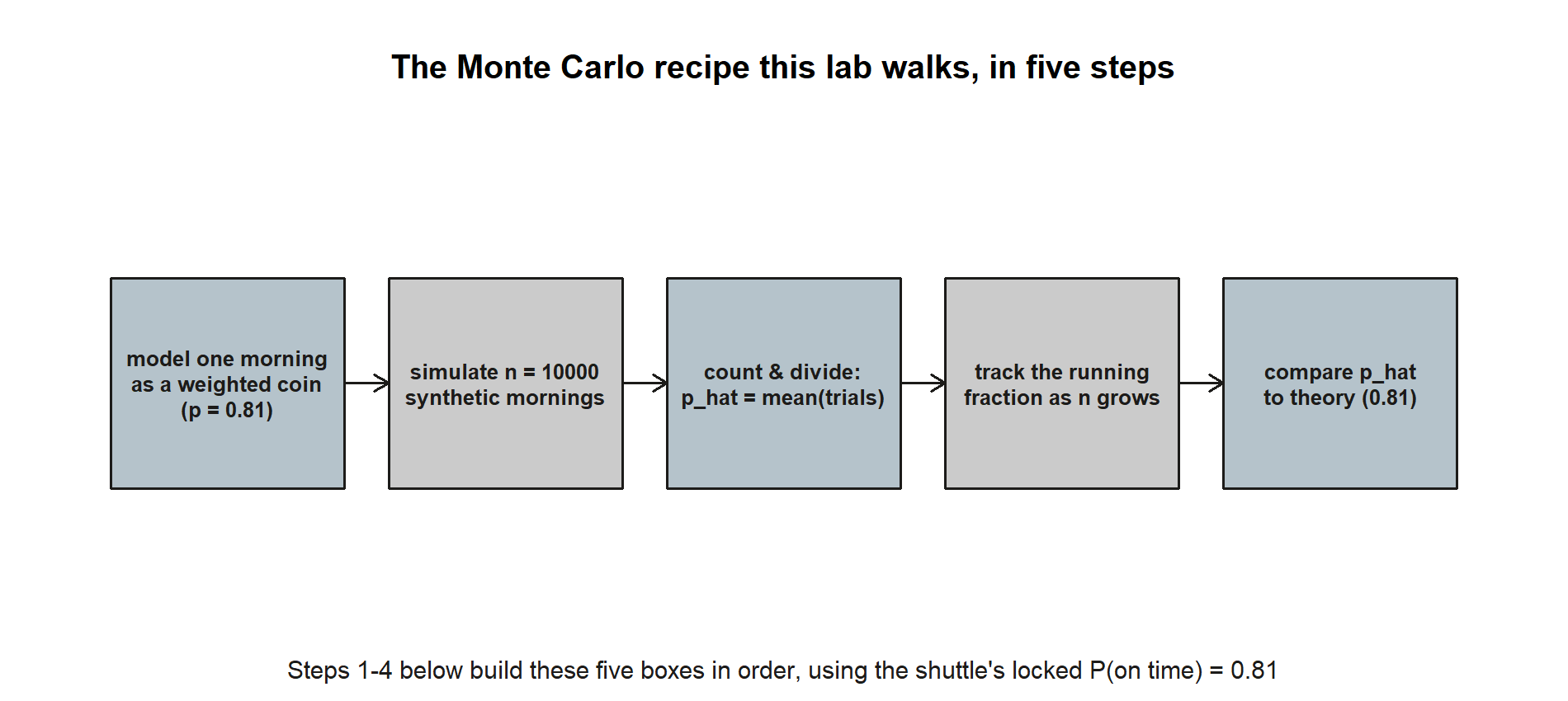
Non-visual equivalent: the recipe in words is (1) model a morning as a weighted coin with \(P(\text{on time})=0.81\), (2) simulate n_trials such mornings, (3) estimate by counting (p_hat = mean(trials)), (4) track the running fraction as more mornings accumulate, (5) compare that running fraction to the theoretical \(0.81\). Steps 1–4 below build exactly these five pieces, in this order.

Goal

By the end of this lab you will be able to:

1. Model a single random trial — one of Maya’s mornings — as a weighted coin flip that lands “on time” with probability \(0.81\) and “late” with probability \(0.19\), using rbinom() with size = 1.
2. Estimate a probability by counting — generate many such trials and take their mean, so that the sample fraction of on-time mornings becomes your Monte Carlo estimate of \(P(\text{on time})\).
3. Watch the estimate converge — compute the running relative frequency as trials accumulate and see it tighten around the theoretical value \(0.81\).
4. Compare simulation to theory — read the gap between your estimate and \(0.81\) as Monte Carlo error, and explain why that gap tends to shrink like \(1/\sqrt{n}\) rather than disappearing all at once.

Everything here is base R. The code is shown for study and is marked so that it does not execute on this site; you run it yourself in your own R session, where the fixed seed makes the output reproducible.

Setup

You need nothing beyond a working R installation and, ideally, the project setup described on the R · Quarto setup page. No add-on packages are required — rbinom(), mean(), cumsum(), and plot() are all part of base R.

The situation we are modeling is the recurring one from the notes. Maya catches a campus shuttle each weekday morning. On any given morning the shuttle is either on time or late, and from the Week 2 and Week 3 development we take the long-run on-time chance as a fixed, known number:

\[ P(\text{on time}) = 0.81, \qquad P(\text{late}) = 1 - 0.81 = 0.19 . \]

We will treat each morning as an independent trial with this fixed success probability — a weighted coin flip where “heads” means on time. That assumption (independent, identically weighted mornings) is exactly what makes the long-run-frequency picture clean, and it is the assumption we are choosing to simulate. The numbers are synthetic; seed 35003 set throughout.

Two small conventions make the code below easy to read:

• We encode each trial as a number: 1 = on time, 0 = late. With that coding, the count of on-time mornings is just the sum of the trials, and the fraction on time is their mean.
• We set the seed once, at the very top of the script, before any random numbers are drawn. Re-running from that line reproduces the entire lab.

# Lab 2 — Monte Carlo basics. Synthetic data; seed set for reproducibility.
set.seed(35003)

p_on_time <- 0.81   # theoretical P(on time) from the Week 2/3 notes
n_trials  <- 10000  # number of synthetic mornings to simulate

Read the two constants as the two things a Monte Carlo study always needs: the truth we are trying to recover (p_on_time, here known, because this is a teaching example) and the amount of effort we will spend (n_trials). In a real application you would not know p_on_time — that is what you would be estimating. We keep it on hand here precisely so we can check the estimate against it at the end.

Steps

Step 1 — Simulate the trials

A single morning is a weighted coin flip. The base-R tool for “flip a coin that lands 1 with probability p” is rbinom(n, size = 1, prob = p): it returns n independent draws, each a 0 or a 1, where 1 appears with probability prob. Setting size = 1 is what makes each draw a single trial (a Bernoulli trial) rather than a count over several flips. Asking for n_trials of them in one call gives us the whole run of synthetic mornings at once.

set.seed(35003)

# Each entry is one morning: 1 = on time, 0 = late.
trials <- rbinom(n = n_trials, size = 1, prob = p_on_time)

# A first look at what we made.
length(trials)      # how many mornings: 10000
head(trials, 20)    # the first 20 mornings as 0s and 1s
sum(trials)         # how many were on time, in total

The vector trials is the simulated long run: ten thousand mornings, each a 0 or a 1. There is nothing mysterious in it — it is just a list of coin flips weighted toward “on time.” sum(trials) counts the on-time mornings, and because on-time is coded 1, that sum is the count of the event we care about. Notice that we call set.seed(35003) again here. That is deliberate: it lets this step stand on its own and reproduce the exact same trials whether or not you ran the setup chunk first.

The chunk above is shown but not executed on this page. Because the seed is fixed, running it yourself produces one exact, reproducible sequence — the figure below shows precisely what that sequence looks like.

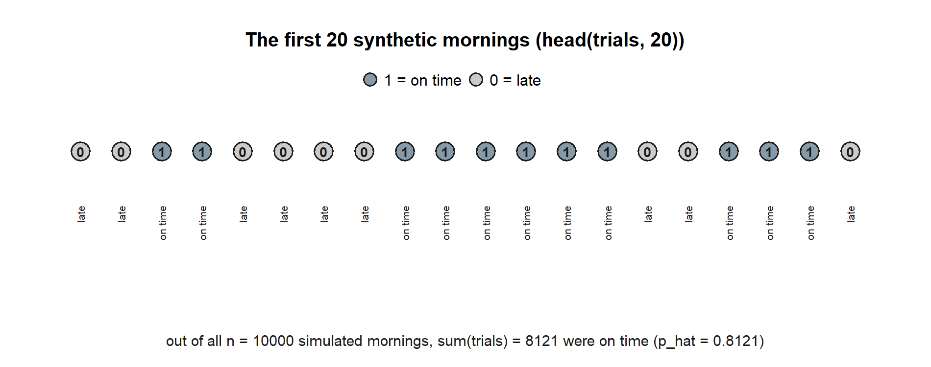
Figure 2: The first 20 synthetic mornings, and the full-run total (synthetic; seed 35003). The strip reproduces head(trials, 20) exactly; the caption line reproduces sum(trials) over all n_trials = 10000 mornings.

Non-visual equivalent: head(trials, 20) is 0 0 1 1 0 0 0 0 1 1 1 1 1 1 0 0 1 1 1 0; sum(trials) over all 10,000 mornings is \(8121\) on-time mornings.

Step 2 — Estimate the probability by counting

The Monte Carlo estimate of \(P(\text{on time})\) is the fraction of mornings that came up on time:

\[ \widehat{P}(\text{on time}) = \frac{\text{number of on-time mornings}}{\text{number of mornings}} = \frac{1}{n}\sum_{i=1}^{n} \text{trial}_i . \]

With our 0/1 coding, that fraction is exactly the mean of the trials vector — summing 1s and dividing by the count is what mean() does. So the estimate is a single, almost anticlimactic line of code.

# The Monte Carlo estimate is just the sample fraction of on-time mornings.
n_on_time <- sum(trials)          # count of the event
p_hat     <- mean(trials)         # equivalently n_on_time / n_trials

n_on_time
p_hat                             # our estimate of P(on time)

p_hat is the lab’s headline number: the simulation’s verdict on how often the shuttle is on time, read off purely by counting and dividing. It will be close to \(0.81\) but, on any finite run, not exactly equal to it. That small gap is not a mistake — it is Monte Carlo error, the price of estimating a probability from a finite sample instead of computing it exactly. The next step shows where that gap comes from and how it behaves as the run grows.

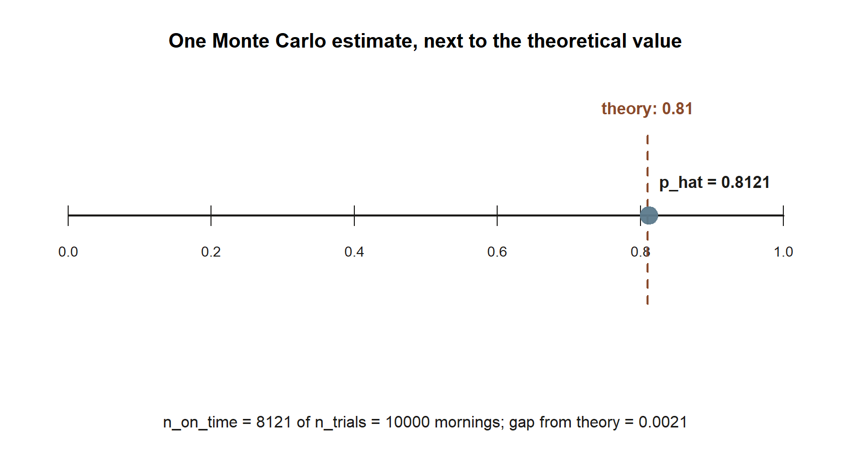
Figure 3: One Monte Carlo estimate, next to the theoretical value (synthetic; seed 35003). The point marks p_hat; the dashed line marks the theoretical p_on_time = 0.81 this run is trying to recover.

Non-visual equivalent: n_on_time = 8121, p_hat = 0.8121, a gap from theory of about \(0.0021\) — a single estimate landing close to, but not exactly on, \(0.81\).

Step 3 — Watch the running relative frequency converge

A single estimate hides the most instructive part of the story: how the fraction settles down as mornings accumulate. To see it, we compute the running relative frequency — after morning 1, after morning 2, after morning 3, and so on — and look at the whole trajectory. The running count of on-time mornings up to each point is a cumulative sum (cumsum), and dividing by the morning index turns each running count into a running fraction.

# Running fraction of on-time mornings after 1, 2, 3, ..., n trials.
running_count <- cumsum(trials)           # on-time mornings so far
index         <- seq_along(trials)        # 1, 2, 3, ..., n_trials
running_freq  <- running_count / index    # the estimate after each morning

# The estimate is volatile early and steadies as n grows.
running_freq[c(10, 100, 1000, 10000)]     # snapshots at four sample sizes

Reading the four snapshots from left to right tells the convergence story in one line: at \(n = 10\) the estimate can be well off, at \(n = 100\) it is closer, and by \(n = 1000\) and \(n = 10000\) it is hugging \(0.81\). Plotting the whole path makes the behavior unmistakable — early wild swings that calm into a near-flat line near the true value.

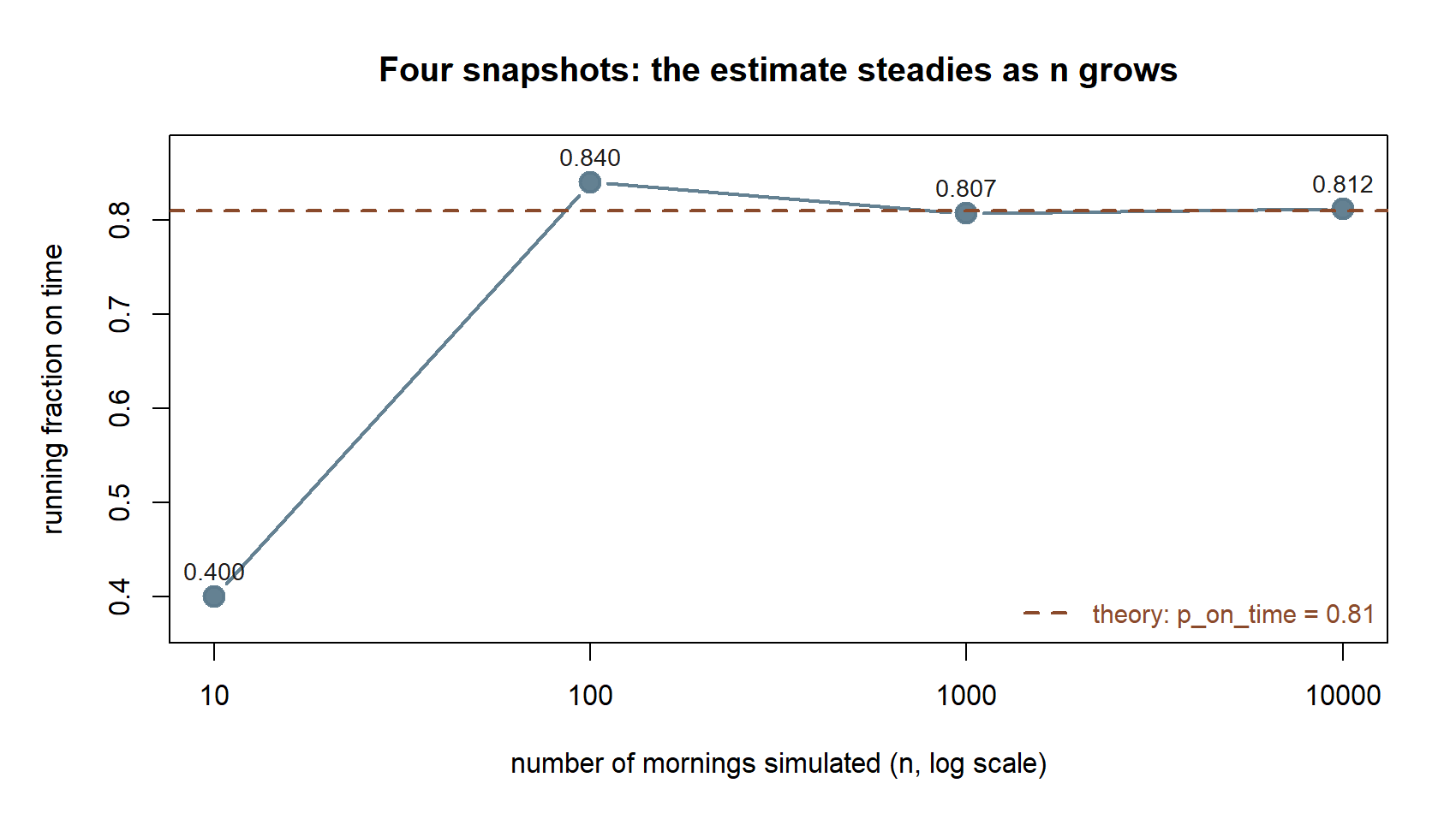
Figure 4: Four snapshots of the running fraction (synthetic; seed 35003). The same running_freq vector, read off at \(n = 10, 100, 1000, 10000\) — coarse frames from the full movie the next figure plays.

Non-visual equivalent: running_freq[c(10, 100, 1000, 10000)] is \(0.400,\ 0.840,\ 0.807,\ 0.812\) — noisy at \(n=10\), then progressively closer to \(0.81\).

plot(index, running_freq, type = "l",
     xlab = "number of mornings simulated (n)",
     ylab = "running fraction on time",
     main = "Monte Carlo estimate settling toward 0.81")
abline(h = p_on_time, lty = 2)            # the theoretical value 0.81

The dashed horizontal line marks the truth, \(0.81\). The solid curve is your estimate as a function of how many mornings you have counted. The shape is the whole lesson: the curve does not march smoothly to the line, it rattles toward it, with the rattling growing quieter as \(n\) grows. The narrowing of those swings is the \(1/\sqrt{n}\) behavior made visible — to halve the typical width of the wiggle you must run roughly four times as many trials.

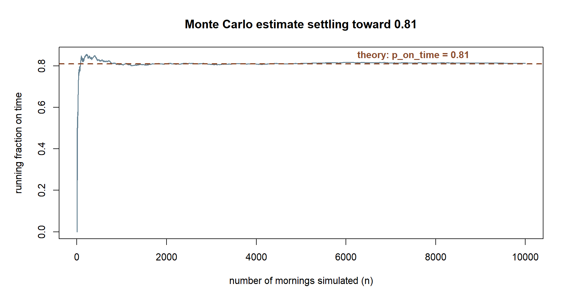
Figure 5: The convergence plot the chunk above would produce (synthetic; seed 35003). This is exactly the plot(index, running_freq, ...) call, run once and captured: wide early swings that visibly narrow and settle against the dashed \(0.81\) line.

Non-visual equivalent: the running fraction swings between roughly \(0.4\) and \(0.85\) within the first few hundred mornings, then settles within about \(\pm 0.01\) of \(0.81\) by \(n \approx 2000\) and stays there.

Step 4 — Compare to the theoretical 0.81

The last step makes the comparison explicit. We report the estimate, the truth, and the gap between them — the realized Monte Carlo error on this run — and put it next to a back-of-envelope sense of how big that gap should be.

# Estimate vs. theory, and the realized error on this run.
abs_error <- abs(p_hat - p_on_time)

c(estimate    = p_hat,
  theoretical = p_on_time,
  abs_error   = abs_error)

# A rough yardstick for the typical error at this n:
# sqrt(p(1-p)/n) is the standard deviation of the estimate.
typical_error <- sqrt(p_on_time * (1 - p_on_time) / n_trials)
typical_error

Two numbers are worth dwelling on. The first is abs_error: how far this particular simulation landed from \(0.81\). The second is typical_error, the quantity \(\sqrt{p(1-p)/n}\), which is the standard deviation of the Monte Carlo estimate — a rule-of-thumb for how far off a run of this size usually is. You should find abs_error is comfortably within a small multiple of typical_error; that is the sense in which the estimate is “as accurate as it should be” for the effort spent. And because \(n\) sits under a square root in typical_error, the message is the same one the convergence plot drew: accuracy improves with more trials, but only as fast as \(1/\sqrt{n}\).

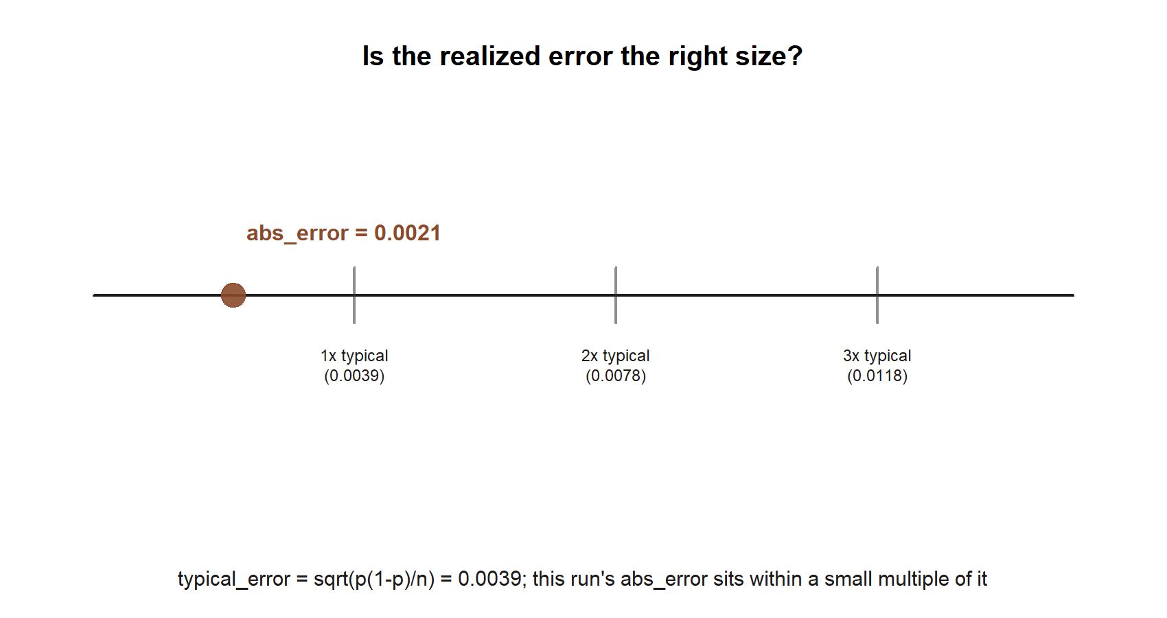
Figure 6: Is the realized error the right size (synthetic; seed 35003)? abs_error placed against 1x, 2x, and 3x of typical_error — the yardstick for deciding whether a gap from theory is ordinary Monte Carlo noise or a sign something is wrong.

Non-visual equivalent: typical_error \(\approx 0.0039\); this run’s abs_error \(\approx 0.0021\), which is about \(0.5\) times typical_error — comfortably inside the “small multiple” you should expect, not zero and not many multiples too large.

A common misreading to avoid: neither an error of exactly zero nor a very large error is the reassuring outcome. Zero would be a suspiciously perfect finite-sample run; several multiples of typical_error would suggest a bug (a mistyped prob, or reusing an already-consumed random stream) rather than ordinary Monte Carlo noise. “Comfortably within a small multiple” is the target, not “as close as possible.”

Verify

A simulation result is trustworthy only if it agrees with something you already know by other means. Here the “other means” is the theory from the notes, and there are three checks worth making before you believe your own output:

1. Does the estimate match the theory? Compare p_hat to \(0.81\). With ten thousand trials they should agree to roughly two decimal places. If p_hat is wildly off — say \(0.5\) or \(0.95\) — suspect the prob argument, not the universe: a mistyped probability is the usual culprit.
2. Does the running frequency settle, not wander? The convergence plot should show large early swings that visibly damp down and hug the dashed line near \(0.81\) as \(n\) grows. A curve that keeps swinging at large \(n\), or drifts toward a different level, means the trials are not what you think they are.
3. Is the realized error the right size? Confirm that abs_error is within a small multiple (say, two or three times) of typical_error \(= \sqrt{p(1-p)/n}\). An error many times larger than that is a red flag; an error of exactly zero on a finite run would be suspicious in the other direction.

A portability check. Nothing about the four steps above is special to \(0.81\). The Week 2 sample space also gives us \(P(\text{rain}) = 0.30\); swap prob = 0.81 for prob = 0.30 in simulate-trials, re-run the identical four steps with the same set.seed(35003), and you should see a running-frequency curve that rattles early and settles — not near \(0.81\) this time, but near \(0.30\). The figure below shows exactly that run, so you can check your own re-run against it before you trust the recipe on a probability of your own choosing.

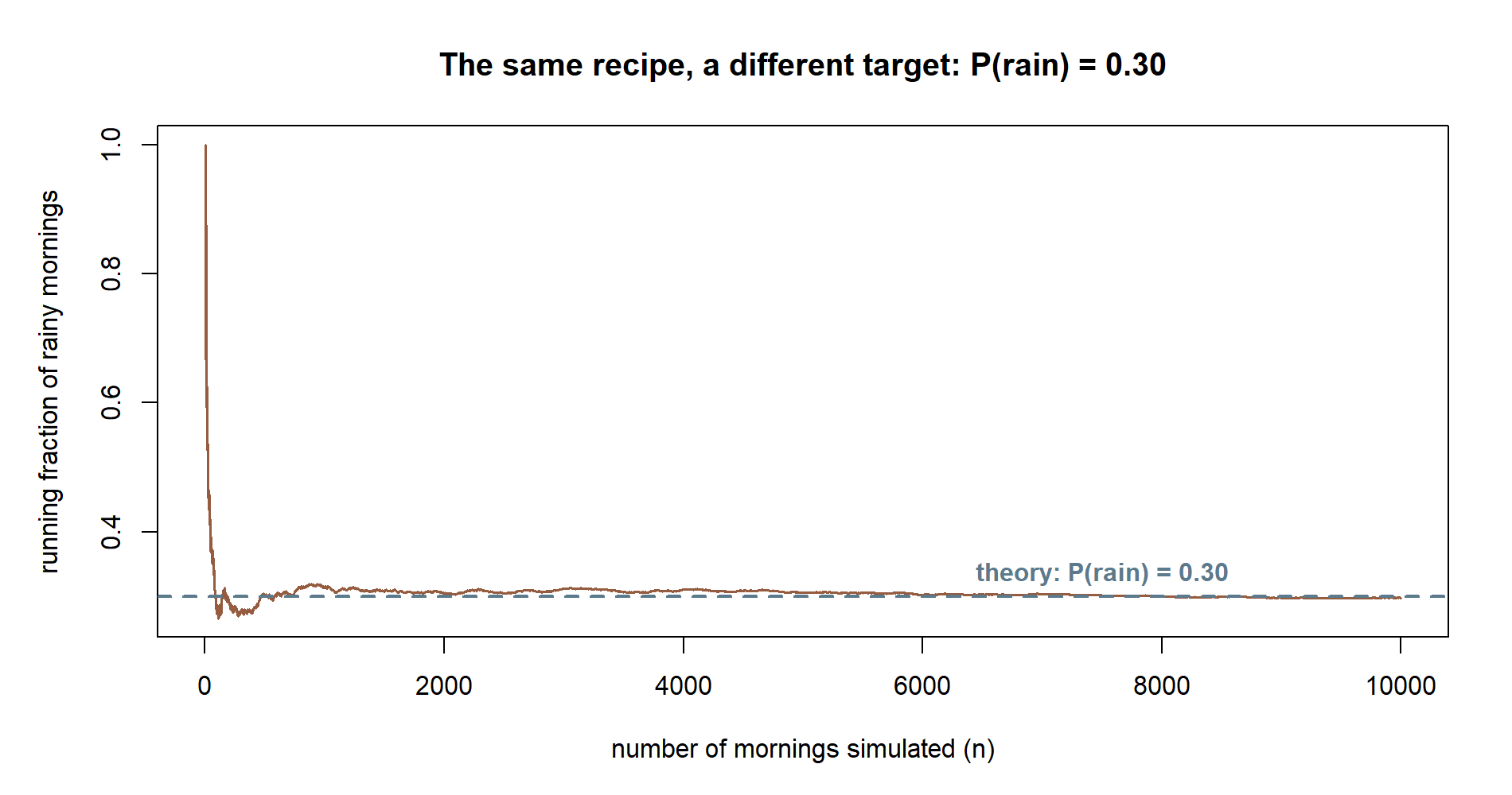
Figure 7: The same recipe, aimed at a different locked probability (synthetic; seed 35003). Everything is identical to the Step 1–4 code except prob = 0.30 in place of prob = 0.81 — the shuttle’s chance of rain, not of being on time.

Non-visual equivalent: with prob = 0.30 and the same n_trials = 10000 and seed, the final running fraction is about \(0.298\) — close to the locked \(P(\text{rain}) = 0.30\), by the identical count-and-divide logic used throughout this lab.

One more reproducibility check ties it all together: run the whole script a second time from set.seed(35003) and confirm you get the identical p_hat, the identical plot, and the identical abs_error. A Monte Carlo result that changes every time you run it is not yet a result — fixing the seed is what makes it one. If a classmate runs your code on their machine and reports a different number, the first thing to check is whether the seed line ran before any random draw.

AI use note

If you use an AI assistant while working through this lab, record it briefly and honestly. The load-bearing column is Verification — what you did to confirm the AI’s output was correct, because you, not the tool, are responsible for the result. Original work is expected; the assistant is a study aid, not an author.

Tool	Purpose	Verification
AI chat assistant	Explain what rbinom(n, size = 1, prob = p) returns and how size = 1 makes a single Bernoulli trial	Read the base-R ?rbinom help page myself; ran a tiny call with prob = 0.5 and checked the mean came out near \(0.5\)
AI chat assistant	Suggest how to compute a running relative frequency in base R	Confirmed cumsum(trials) / seq_along(trials) against a hand-checked first three entries; checked the final entry equals mean(trials)
AI coding helper	Draft the convergence-plot call	Compared the plotted limit to the theoretical \(0.81\) via the dashed abline(h = ...); re-ran from set.seed(35003) to confirm the figure was reproducible

See also

• Week 2 — Sample spaces, events & rules — the companion note, where \(P(\text{on time}) = 0.81\) is defined and read as a long-run frequency.
• Lab 5 — Bayes by simulation — the same count-and-divide idea taken one step further, to recover a conditional (posterior) probability by simulating a whole population.
• R · Quarto setup — how to get R, RStudio/Posit Cloud, and Quarto running so you can execute these chunks yourself.
• Distribution reference — a quick reference for the base-R random-draw functions, including rbinom and the Bernoulli/Binomial parameterization used here.

The graded deliverable, its rubric, and due date live in Blackboard (the LMS) — this page is study and practice only.