Lab 9 — Simulating discrete models

Generating draws from binomial and Poisson models and comparing to the formulas

Purpose. This lab puts the named discrete models from Week 9 — Common discrete models on the computer. There you learned to read a probability, a mean, and a variance straight off a model’s parameters. Here you generate draws from those same models and check, by counting, that the empirical frequencies land where the formulas say they should. Seeing the two agree — formula and simulation — is the point.

The idea

In the Week 9 note you committed to a habit: name the model, state its assumptions, then read its probabilities off the parameters. A binomial count of correct guesses, a Poisson count of shuttle arrivals — each came with an exact pmf, an exact mean, and an exact variance. That note did the arithmetic by hand.

A simulation does something complementary. Instead of summing pmf terms, it manufactures the random variable: it asks R to play the experiment out tens of thousands of times and then counts how often each result occurred. If your model is right, the long-run relative frequency of an event settles toward the probability the formula gives, and the average and spread of the simulated draws settle toward the model’s mean and variance. This is the same Monte Carlo logic you met in Lab 2 — Monte Carlo basics, now aimed at two named models rather than a single hand-built experiment.

Why bother, when you already have the exact answers? Three reasons. First, agreement between an independent simulation and a hand calculation is a genuine check on both — a typo in the formula or a misread parameter usually shows up as a mismatch. Second, the simulation makes the variability tangible: you watch four arrivals an hour fail to be exactly four most of the time, instead of just being told the variance is four. Third, when a problem gets too tangled to sum by hand, simulation is often the only practical route to an answer — so it is worth trusting it on cases you can check by hand first. That is exactly what this lab does: every simulated quantity has a formula answer sitting next to it, so you can see the method working before you ever rely on it blind.

A note on what the simulation can and cannot tell you. A simulated relative frequency is itself a random quantity — run it again with a different seed and you get a slightly different number. It approximates the true probability, and the approximation gets tighter as you draw more samples, but it never lands exactly on the formula value. So “close” is the standard you are checking against, not “identical.” Part of the skill this lab builds is developing a feel for how close is close enough, and for why a hundred thousand draws gives a steadier answer than a hundred.

Goal

By the end of this lab you should be able to:

• Generate many independent draws from a binomial model with rbinom() and from a Poisson model with rpois(), with a fixed seed so the run is reproducible.
• Estimate a tail probability, a mean, and a variance from simulated draws by counting and averaging, and compare each estimate to the exact formula value from the Week 9 note.
• Confirm the binomial quiz result \(P(X \ge 8) \approx 0.0547\), the mean of \(5\), and the variance of \(2.5\) by simulation, and the Poisson result \(P(N = 4) \approx 0.195\) with mean and variance both near \(4\).
• Explain why R’s *geom family uses a different geometric convention than the course (failures before the first success, support starting at \(0\)) and adjust for it.
• Judge whether a simulated estimate is “close enough” to its formula value, and say what makes it closer.

All data in this lab are synthetic; seed 35003 is set in every simulation chunk so your run reproduces.

Setup

You need a working R session with Quarto — see R · Quarto setup if you have not set one up yet. Everything here is base R; no packages to install. The four functions you will lean on are part of R’s built-in distribution family:

• rbinom(n, size, prob) — draw n binomial counts, each the number of successes in size independent trials with success probability prob.
• rpois(n, lambda) — draw n Poisson counts, each with rate (mean) lambda.
• mean() and var() — the sample average and sample variance of a vector of draws.
• a logical comparison such as x >= 8 or y == 4, which R turns into TRUE/FALSE; wrapping it in mean() gives the proportion that are TRUE, i.e. an estimated probability.

That last trick is the engine of the whole lab, so it is worth pausing on. In R, TRUE counts as \(1\) and FALSE as \(0\). So mean(x >= 8) adds up one for every draw that clears \(8\) and divides by how many draws there were — exactly the relative frequency of the event \(\{X \ge 8\}\). Estimating a probability becomes a one-line mean() of a comparison.

Two quantities to fix before you start, both straight from the Week 9 note. The quiz model is \(X \sim \text{Binomial}(10, 0.5)\) — ten true/false questions, each guessed correctly with probability \(0.5\). The arrivals model is \(N \sim \text{Poisson}(4)\) — shuttle arrivals in an hour at a rate of four per hour. Keep the formula targets in view as you go, because the whole exercise is comparison:

\[ P(X \ge 8) = \frac{56}{1024} \approx 0.0547, \qquad E[X] = 5, \qquad \operatorname{Var}(X) = 2.5, \]

\[ P(N = 4) = \frac{e^{-4}\,4^{4}}{4!} \approx 0.195, \qquad E[N] = \operatorname{Var}(N) = 4. \]

Pick a sample size large enough to make the relative frequencies steady. This lab uses \(100{,}000\) draws throughout; smaller runs work but wobble more, which is itself something worth seeing (the last step asks you to try it).

Steps

The R chunks below are shown for study — they carry #| eval: false, so they are not executed on this site. Read each chunk, make sure you can say what every line does, then run it yourself in your own R session. Every chunk sets set.seed(35003) so your numbers reproduce.

Every step below walks the same four-box path: start from the formula, simulate a hundred thousand draws, summarize them, and compare. Keeping that shape in mind makes each step a variation on one habit rather than four unrelated recipes.

Figure 1: The four-step path every step in this lab follows: formula, simulate, summarize, compare. Synthetic; seed 35003.

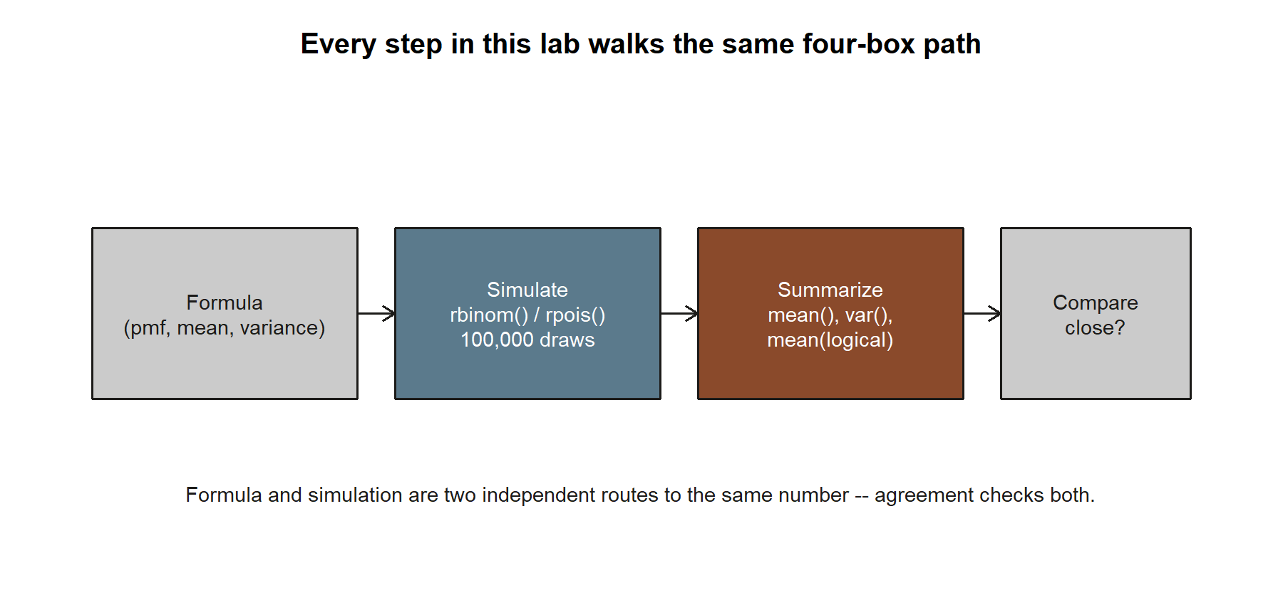
This diagram is not a new step — it names the shape that Steps 1 through 4 already share. Wherever a step asks you to compare a simulated number to a formula value, it is walking these same four boxes.

Step 1 — Draw from the binomial quiz model and check mean and variance

Start with the quiz. Generate one hundred thousand independent plays of the ten-question quiz, where each play returns the number of correct guesses out of ten. Then check that the simulated average and variance match the formula values \(5\) and \(2.5\).

set.seed(35003)

n_sim <- 100000

# each draw is the number correct in 10 fair-guess true/false questions
x <- rbinom(n_sim, size = 10, prob = 0.5)

# the simulated distribution of scores, as a quick sanity check
table(x)

# compare to the formula values from the Week 9 note
mean(x)   # should sit close to E[X]  = n*p       = 5
var(x)    # should sit close to Var(X)= n*p*(1-p) = 2.5

A few things to notice in the output. table(x) shows the shape of the binomial — counts bunched around \(5\), thinning out toward \(0\) and \(10\), symmetric because \(p = 0.5\). The mean(x) should print something very close to \(5\) and var(x) something very close to \(2.5\). They will not be exactly \(5\) and \(2.5\): these are sample statistics from a finite run, so expect agreement to two or three figures, not perfect equality. If mean(x) came back near \(2.5\) instead of \(5\), that would be a red flag — almost certainly a wrong size or prob, not bad luck. The numbers being in the right neighborhood is the check; the small wobble is normal.

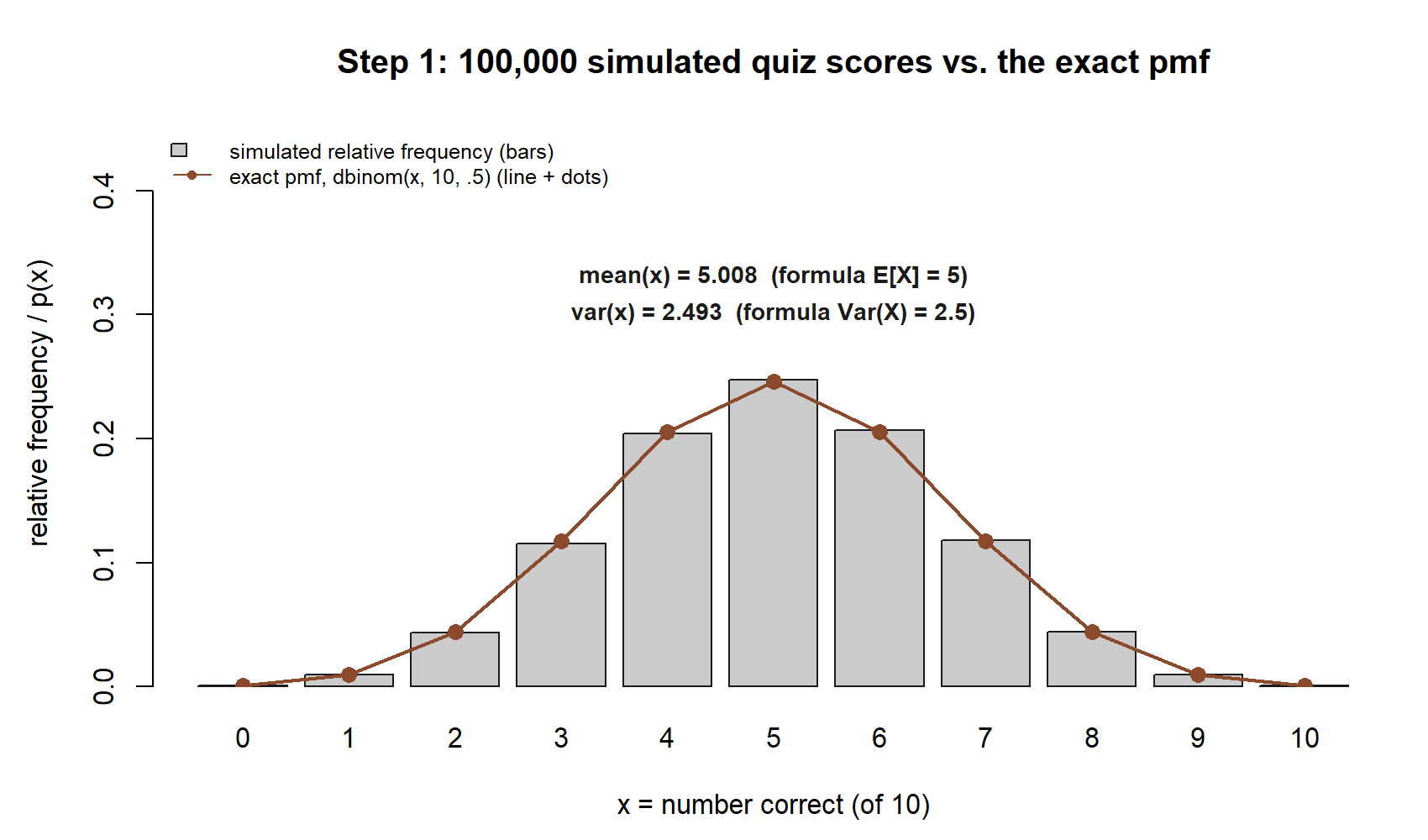
Figure 2: The 100,000 simulated quiz scores (bars) against the exact pmf (line and dots), with the run’s own mean(x) and var(x) shown against the formula values \(5\) and \(2.5\). Synthetic; seed 35003.

What this shows. The bars (what the simulation produced) and the line (what the formula predicts) sit almost exactly on top of each other at every score from \(0\) to \(10\) — that overlap is the check table(x), mean(x), and var(x) are asking you to make. The non-visual equivalent is the run’s own printed numbers: mean(x) and var(x) next to the formula’s \(5\) and \(2.5\).

Step 2 — Estimate the binomial tail probability \(P(X \ge 8)\)

Now reproduce the headline result from the note: the chance a pure guesser scores at least eight out of ten. The formula gives \(56/1024 \approx 0.0547\). The simulation estimates it by counting the fraction of draws that clear eight.

set.seed(35003)

n_sim <- 100000
x <- rbinom(n_sim, size = 10, prob = 0.5)

# P(X >= 8): the fraction of plays scoring 8, 9, or 10
mean(x >= 8)          # should sit close to 56/1024 = 0.0547

# break it down to see where the mass sits
mean(x == 8)          # ~ 45/1024 ~ 0.0439
mean(x == 9)          # ~ 10/1024 ~ 0.0098
mean(x == 10)         # ~  1/1024 ~ 0.0010

# and confirm the exact target the estimate is chasing
56 / 1024             # 0.0546875

The line mean(x >= 8) is the whole estimate: it asks, of one hundred thousand plays, what fraction scored eight or higher, and that fraction should land near \(0.0547\). Breaking it into x == 8, x == 9, and x == 10 shows the same structure the formula used — the \(45\), \(10\), and \(1\) arrangements over \(1024\) — now appearing as three relative frequencies that add up to the tail. Because \(P(X \ge 8)\) is a small probability, it is the noisiest estimate in this lab: a rare event needs more draws to pin down than a common one, which is why a hundred thousand plays (not a hundred) is worth the wait here. Confirm your simulated value rounds to about \(0.055\) and you have matched the note by an independent route.

Figure 3: The exact pmf (bars, with \(x \ge 8\) highlighted) against the simulated relative frequency (open circles) at every score. Synthetic; seed 35003.

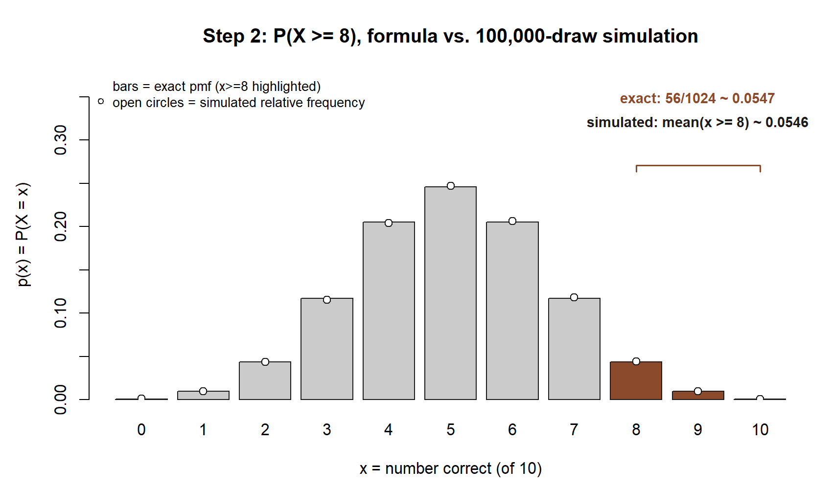
What this shows. The highlighted bars are the same three bars (\(8\), \(9\), \(10\)) the note summed by hand; the open circles are where \(100{,}000\) simulated plays actually landed. Formula (\(\approx 0.0547\)) and simulation (\(\approx 0.0546\)) land within a thousandth of each other — the kind of agreement Step 2 asks you to confirm without a picture, here made visible.

Step 3 — Draw from the Poisson arrivals model and check \(P(N = 4)\) and the mean–variance equality

Switch to the shuttle-arrivals model, \(N \sim \text{Poisson}(4)\). Generate one hundred thousand hours of arrivals, estimate the chance of exactly four arrivals in an hour, and confirm the Poisson signature that mean and variance are both near the rate \(\lambda = 4\).

set.seed(35003)

n_sim <- 100000

# each draw is the number of shuttle arrivals in one hour at rate lambda = 4
y <- rpois(n_sim, lambda = 4)

# the simulated distribution of hourly counts
table(y)

# P(N = 4): the fraction of hours with exactly four arrivals
mean(y == 4)          # should sit close to e^-4 * 4^4 / 4! ~ 0.195

# the Poisson signature: mean and variance both near lambda = 4
mean(y)               # ~ 4
var(y)                # ~ 4

# the exact target the P(N=4) estimate is chasing
exp(-4) * 4^4 / factorial(4)   # 0.1953668

The mean(y == 4) line estimates \(P(N = 4)\) the same way Step 2 estimated the binomial tail — the fraction of draws equal to four — and it should land near \(0.195\). Notice that even though four per hour is the average, exactly four happens under a fifth of the time; the rest of the probability spreads over three, five, two, six, and beyond. That spread is the variance at work. The pair mean(y) and var(y) should both sit near \(4\): this near-equality is the Poisson’s fingerprint, and seeing it in simulated data is a quick way to gauge whether a real count dataset is plausibly Poisson. If the simulated variance came out much larger than the mean — say near \(10\) while the mean stayed near \(4\) — that would signal the steady-independent-rate story was violated, exactly the diagnostic the note described.

Figure 4: The 100,000 simulated hourly arrival counts (bars, with \(y = 4\) in iron) against the exact Poisson(4) pmf (dashed line and dots). Synthetic; seed 35003.

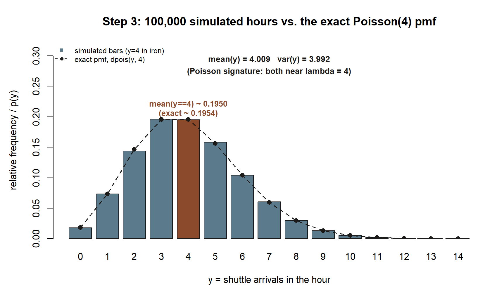
What this shows. The highlighted bar at \(y = 4\) is the single tallest bar, but most of the shaded area belongs to the other bars — a picture of “four is the average, not the guarantee.” The overlaid dashed curve is the exact pmf; the fact that it sits almost on top of the simulated bars is the same agreement mean(y == 4) reports as a number, and mean(y) next to var(y) is the Poisson signature (both near \(4\)) read straight off the plot’s title numbers.

Step 4 — Mind the geometric convention, and feel the role of sample size

This step has two short parts, both about not being misled.

Part A — R’s geometric counts differently than the course. The Week 9 note fixed the course’s geometric as the number of trials up to and including the first success, so its support starts at \(1\). R’s *geom family — rgeom, dgeom, pgeom — instead counts the number of failures before the first success, so its support starts at \(0\). The two differ by exactly one. If you simulate a “waiting for the first success” count with rgeom and forget this, every value is one too small and your estimated mean comes out as \(\frac{1}{p} - 1\) instead of \(\frac{1}{p}\). The fix is to add one:

set.seed(35003)

n_sim <- 100000
p <- 0.25

# R's rgeom: FAILURES before the first success, support starts at 0
r_failures <- rgeom(n_sim, prob = p)
mean(r_failures)          # ~ (1 - p)/p = 3   (this is NOT the course's mean)

# convert to the COURSE convention: trials up to and INCLUDING the first success
trials <- r_failures + 1  # now support starts at 1
mean(trials)              # ~ 1/p = 4         (this matches the note's E[X] = 1/p)

The takeaway is not arithmetic; it is a habit. Before you trust any simulated quantity, confirm the function’s convention matches the course’s. rbinom and rpois happen to agree with the note’s parameterizations, so Steps 1–3 needed no adjustment; rgeom does not, so it needs the + 1. The Distribution reference lists each model’s R function and flags this geometric shift explicitly.

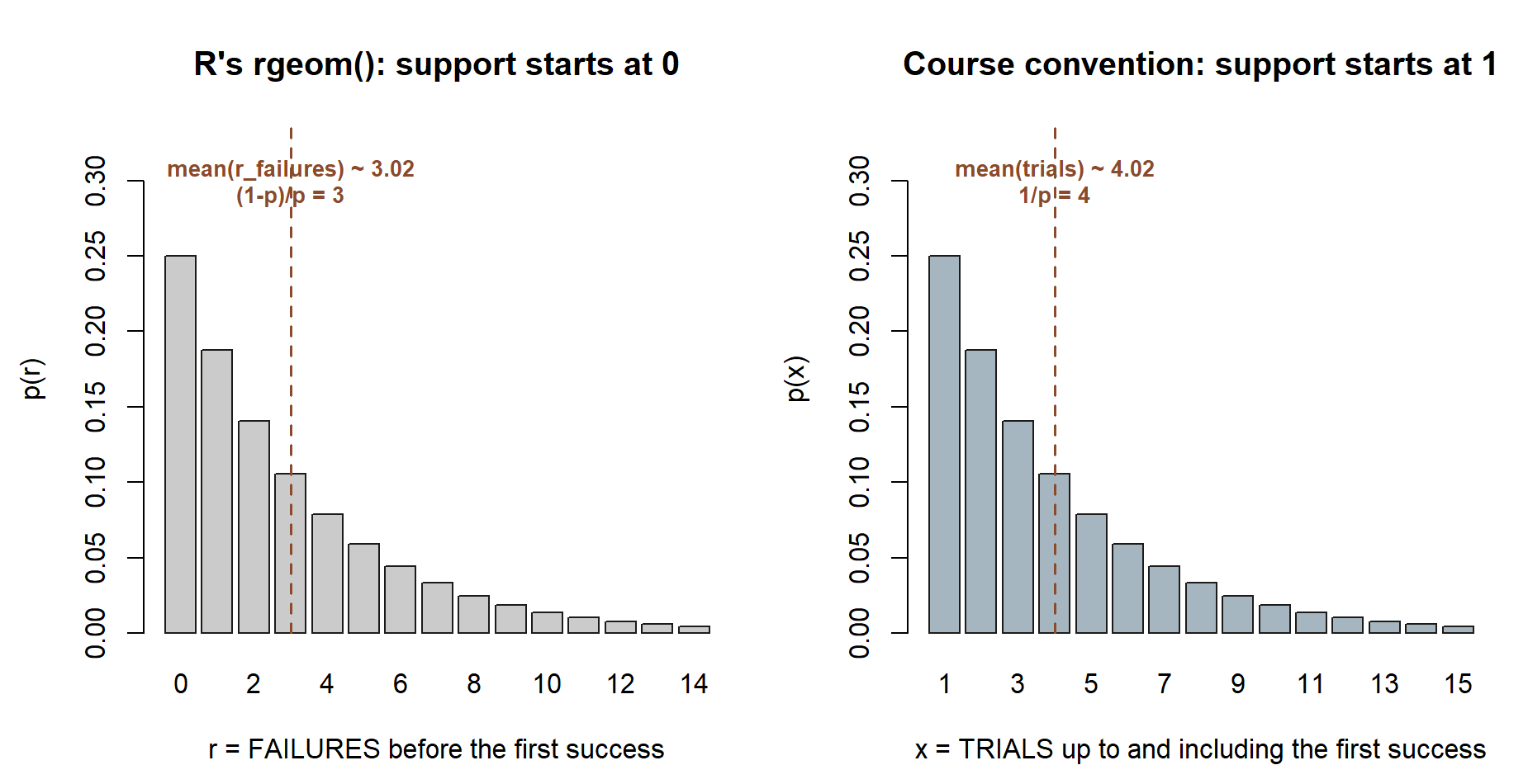
Figure 5: R’s rgeom() convention (failures before the first success, support starting at \(0\), left panel) against the course convention (trials up to and including the first success, support starting at \(1\), right panel), both at \(p = 0.25\). Synthetic; seed 35003.

What this shows. The two panels are the identical shape, shifted by exactly one trial — that shift is the whole convention pitfall in one picture. The left panel’s mean lands near \(3\) (R’s own convention); only after adding \(1\) does the right panel’s mean land near \(4\), matching the course’s \(E[X] = 1/p\). If you ever see a simulated geometric mean sitting one unit low, this is the picture to check against.

Part B — sample size controls the wobble. Re-run the binomial tail estimate from Step 2 at a few different sample sizes and watch the estimate steady up as the sample grows. Smaller runs scatter more widely around \(0.0547\); larger runs hug it.

set.seed(35003)

target <- 56 / 1024   # 0.0546875, the exact value the estimates chase

for (n_sim in c(100, 1000, 10000, 100000)) {
  x <- rbinom(n_sim, size = 10, prob = 0.5)
  est <- mean(x >= 8)
  cat("n =", n_sim, " estimate =", round(est, 4),
      " error =", round(est - target, 4), "\n")
}

At \(n = 100\) the estimate can be off in the second decimal place — sometimes there are simply not enough high-scoring plays to pin a rare event down. By \(n = 100{,}000\) it should track \(0.0547\) closely. This is the law-of-large-numbers idea you will meet head-on in Lab 13 — Law of large numbers and CLT: more draws, steadier estimate. For now it explains why this lab used a hundred thousand draws — small simulations are honest but noisy, and a tail probability needs the larger run to be convincing.

Figure 6: Two hundred replicate estimates of \(P(X \ge 8)\) at each sample size (boxes), the page’s own single seed-35003 run overlaid (diamonds), and the exact target \(56/1024\) (dashed line). Synthetic; seed 35003.

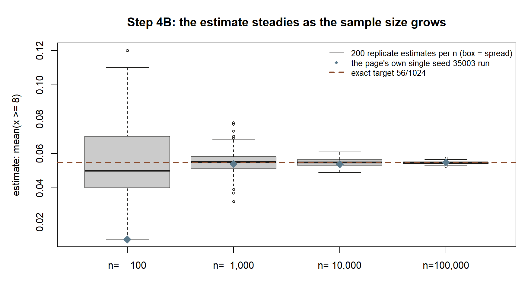
What this shows. Each box is two hundred independent replays of the exact same experiment at one sample size — its height is the wobble the page’s text describes. At \(n = 100\) the box spans roughly \(0.01\) to \(0.12\), wide enough to occasionally miss the target badly (the diamond there, from the page’s own seed-35003 run, is a low outlier); by \(n = 100{,}000\) the box has collapsed to a sliver hugging the dashed target line. The diamonds are exactly the four numbers the shown sample-size-wobble chunk would print if you ran it — the boxes are the added picture of how much another seed could have differed.

Verify

Line up each simulated quantity against the formula value from the Week 9 note and confirm they agree to a sensible number of figures. You are checking for closeness, not exact equality — a finite simulation always carries a little noise.

Quantity	Formula value (Week 9)	What the simulation should show
\(E[X]\), binomial quiz	\(np = 5\)	mean(x) near \(5\)
\(\operatorname{Var}(X)\), binomial quiz	\(np(1-p) = 2.5\)	var(x) near \(2.5\)
\(P(X \ge 8)\)	\(56/1024 \approx 0.0547\)	mean(x >= 8) near \(0.055\)
\(P(N = 4)\), Poisson arrivals	\(e^{-4}4^{4}/4! \approx 0.195\)	mean(y == 4) near \(0.195\)
\(E[N]\) and \(\operatorname{Var}(N)\)	both \(= 4\)	mean(y) and var(y) both near \(4\)
Geometric mean, course convention	\(1/p = 4\) at \(p = 0.25\)	mean(rgeom(...) + 1) near \(4\)

If every row matches to two or three figures, the simulation and the formulas have confirmed each other, and you can trust the method on a problem where you cannot sum by hand. If a row is badly off — not just noisy but in the wrong neighborhood — treat it as a signal, not a fluke: re-check the size, prob, or lambda you passed, confirm you used the right comparison (>= vs ==), and for any geometric work confirm you added the + 1. A good final habit: re-run a chunk with a different seed and confirm the estimate moves only a little. A quantity that swings wildly between seeds at \(n = 100{,}000\) is telling you something is wrong with the setup, not with chance.

AI use note

If you use an AI assistant while working through this lab, keep a short record like the one below. The load-bearing column is Verification — how you confirmed the output was right, independent of the tool. An AI can produce R that runs cleanly and still computes the wrong thing; the formula targets in this lab are exactly what let you catch that.

Tool	Purpose	Verification
AI chat assistant	Explain why mean(x >= 8) estimates a probability	Re-derived it by hand: TRUE counts as \(1\), so the mean is the fraction of draws clearing \(8\); confirmed it tracked \(56/1024 \approx 0.0547\)
AI chat assistant	Draft the rpois chunk for the arrivals model	Checked mean(y) and var(y) both landed near \(4\) and mean(y == 4) near \(0.195\) before trusting the code; confirmed lambda = 4 was passed
AI coding helper	Remind me of R’s geometric convention	Did not take the answer on faith — ran mean(rgeom(n, p)) and saw it gave \((1-p)/p\), confirming the + 1 shift to the course’s mean \(1/p\)

If you used no AI for a step, write “none” — an honest empty record is the correct record.

See also

• Week 9 — Common discrete models — the companion note, where the binomial and Poisson pmfs, means, variances, and the \(P(X \ge 8)\) and \(P(N = 4)\) results are derived by hand.
• Lab 2 — Monte Carlo basics — the earlier lab that introduced estimating a probability by repeated trials and counting, the engine this lab reuses.
• Distribution reference — each model’s pmf, mean, variance, support, and R function in one table, including the geometric support shift between R and the course.
• R · Quarto setup — how to get a reproducible R + Quarto session running before you start.

The graded deliverable, its rubric, and due date live in Blackboard (the LMS) — this page is study and practice only.