Week 11 — Common continuous models

Uniform, exponential, and normal

The week question

Last week you learned the grammar of continuous random variables: a density \(f(x)\) that is not itself a probability, and probability that lives in the area under that density rather than at any single point. That grammar is general, but in practice you do not draw a fresh density for every problem. Just as the discrete world collapsed into a handful of named shapes — Bernoulli, binomial, geometric, Poisson — the continuous world is dominated by a small family of recurring models, each with a one-line story and a formula for its density, mean, and standard deviation.

So this week’s question is: which named continuous model fits a given measurement, and how do you turn that model into a probability? We work through three models that cover an enormous share of first-course problems — the uniform, the exponential, and the normal — and we state the parameterization out loud each time. Continuous models are where the classic convention traps live (rate versus mean, standard deviation versus variance), so naming the convention is not pedantry; it is the difference between a right answer and a plausible-looking wrong one.

Why this matters

A named continuous model carries the same gift its discrete cousin did: say “this is Normal(22, 5)” and you have committed to a specific density, mean, standard deviation, and set of modeling assumptions all at once. You no longer integrate a fresh density by hand for every waiting time or measurement — you recognize the shape, read off the area you need, and interpret it.

But continuous models raise the stakes on one habit: stating the parameterization. Two sources can both write “Exponential(\(\lambda\))” and mean opposite things — one means \(\lambda\) is the rate (so the mean is \(1/\lambda\)), the other means \(\lambda\) is the mean. Two can both write “Normal(\(\mu\), \(\sigma\))” and disagree about whether the second slot is the standard deviation or the variance. Plug a mean into a rate slot, or a variance into a standard-deviation slot, and the formula still renders, still runs, and still returns a confident number — just the wrong one. This is the continuous version of last week’s lesson that a clean-looking calculation can be quietly false.

This course fixes its conventions once and uses them everywhere. Exponential(\(\lambda\)) means \(\lambda\) is a rate, with mean \(1/\lambda\). Normal(\(\mu\), \(\sigma\)) means \(\mu\) is the mean and \(\sigma\) is the standard deviation, not the variance. We restate these in each worked example — partly for discipline, and partly because Maya’s commuter world, shuttle waits and commute times, is exactly where the conventions bite.

Learning goals

By the end of this week you should be able to:

• State the one-sentence story behind the uniform, exponential, and normal models, and say exactly what each one’s parameter(s) mean — including which slot is a rate, a mean, or a standard deviation.
• Write down the density of each model and use it (or its cdf) to find a probability such as \(P(a \le X \le b)\) or \(P(X \le c)\).
• Read off the mean and standard deviation of each model from its parameters, without re-integrating.
• Connect the exponential waiting time to last week’s Poisson count: they describe the same arrival process from two angles.
• Standardize a normal variable, \(Z = (X - \mu)/\sigma\), and use \(\Phi\) to turn a normal question into a standard-normal area.

Core vocabulary

• Uniform model — a continuous variable equally likely to land anywhere in an interval \([a, b]\), with a flat density on that interval and zero outside it. Written \(X \sim \text{Uniform}(a, b)\).
• Exponential model — the continuous waiting time until the next event in a steady-rate, independent arrival process. Written \(T \sim \text{Exponential}(\lambda)\), where \(\lambda\) is the rate (events per unit time) and the mean wait is \(1/\lambda\).
• Rate \(\lambda\) — for the exponential, the average number of events per unit time. It is the same \(\lambda\) that was the Poisson’s mean count per window last week; the waiting time and the count are two views of one process.
• Normal model — the symmetric, bell-shaped “measurement” model. Written \(X \sim \text{Normal}(\mu, \sigma)\), where \(\mu\) is the mean (the center) and \(\sigma\) is the standard deviation (the spread), not the variance.
• Standard normal \(Z\) — the special case \(\text{Normal}(0, 1)\), mean \(0\) and standard deviation \(1\). Every normal question reduces to a standard-normal question by standardizing.
• Standard normal cdf \(\Phi\) — the function \(\Phi(z) = P(Z \le z)\), the area under the standard normal density to the left of \(z\). It has no elementary closed form, so you read it from a table or software, but it is the workhorse for every normal probability.

A convention note you will need all term: this course writes the exponential by its rate \(\lambda\), so a larger \(\lambda\) means events come faster and the mean wait \(1/\lambda\) is shorter; and it writes the normal by its mean and standard deviation, so the second slot of \(\text{Normal}(\mu, \sigma)\) is \(\sigma\), never \(\sigma^2\). (R follows both choices: rexp takes a rate, and rnorm takes mean and sd. We flag this again in the distribution reference.)

Concept development

Uniform — equally likely across an interval

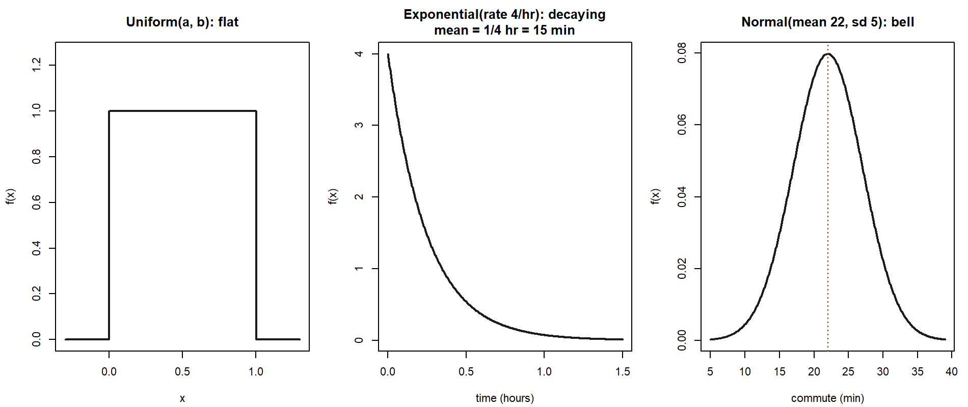
The simplest continuous model says every point in an interval is as likely as every other. If \(X\) is \(\text{Uniform}(a, b)\), its density is flat on \([a, b]\) and zero elsewhere. Because total area must be \(1\) and the base has length \(b - a\), the constant height is forced to be \(1/(b - a)\):

\[ f(x) = \begin{cases} \dfrac{1}{\,b - a\,}, & a \le x \le b, \\[4pt] 0, & \text{otherwise.} \end{cases} \]

Probabilities are then just fractions of the interval, because area under a flat density is height times width. For any sub-interval \([c, d]\) inside \([a, b]\),

\[ P(c \le X \le d) = \frac{d - c}{\,b - a\,}. \]

By symmetry the mean sits at the midpoint, and the spread works out to

\[ E[X] = \frac{a + b}{2}, \qquad \text{Var}(X) = \frac{(b - a)^2}{12}, \qquad \sigma = \frac{b - a}{\sqrt{12}}. \]

The uniform is the right model when you have genuinely no reason to prefer any part of an interval over any other — a rounding error anywhere in a half-unit window, a point dropped at random along a line. It is also the engine behind simulation: the random numbers a computer generates are, at bottom, \(\text{Uniform}(0, 1)\) draws, which is why the uniform underlies nearly every Monte Carlo method in the labs.

Exponential — waiting time at a steady rate

Last week the Poisson counted how many events land in a fixed window when events arrive at a steady average rate \(\lambda\), independently. Turn the same process sideways: starting now, how long until the next event? That waiting time \(T\) is continuous, can be any positive number, and follows the exponential model with the same rate \(\lambda\). Its density is

\[ f(t) = \lambda\, e^{-\lambda t}, \qquad t \ge 0, \]

and the cdf — the probability the wait is at most \(t\) — has a clean closed form you will use constantly:

\[ F(t) = P(T \le t) = 1 - e^{-\lambda t}, \qquad t \ge 0. \]

The mean and standard deviation both come out equal to \(1/\lambda\):

\[ E[T] = \frac{1}{\lambda}, \qquad \sigma = \frac{1}{\lambda}. \]

Notice the parameterization once more: \(\lambda\) is a rate, measured in events per unit time, and the mean wait is its reciprocal \(1/\lambda\), so doubling the rate halves the average wait. The exponential has a famous memoryless property — having already waited a while tells you nothing about how much longer you must wait — which is just what “steady, independent arrivals” should feel like. It is the natural model for the time between independent arrivals: the gap until the next shuttle, customer, phone call, or decay.

Normal — the bell curve for measurements

The third model is the most famous in all of probability: the normal, the symmetric bell curve, parameterized by its mean \(\mu\) (the center) and its standard deviation \(\sigma\) (the spread), with density

\[ f(x) = \frac{1}{\sigma \sqrt{2\pi}}\, e^{-\frac{(x - \mu)^2}{2\sigma^2}}, \qquad -\infty < x < \infty, \]

and, by construction,

\[ E[X] = \mu, \qquad \sigma_X = \sigma, \qquad \text{Var}(X) = \sigma^2. \]

The density never closes into an elementary antiderivative, so you cannot integrate it by hand to get a probability. Instead you standardize. Subtract the mean and divide by the standard deviation to turn any normal \(X\) into the standard normal \(Z \sim \text{Normal}(0, 1)\):

\[ Z = \frac{X - \mu}{\sigma}, \qquad P(X \le c) = P\!\left(Z \le \frac{c - \mu}{\sigma}\right) = \Phi\!\left(\frac{c - \mu}{\sigma}\right). \]

The quantity \(z = (c - \mu)/\sigma\) is a \(z\)-score: it says how many standard deviations \(c\) sits above (or below) the mean. Once you have a \(z\)-score, the single function \(\Phi(z) = P(Z \le z)\) — read from a table or software — gives the area, and every normal probability reduces to looking up \(\Phi\). The normal earns its ubiquity because it emerges whenever many small, independent influences add up: measurement errors, heights, and — as Week 13 will make precise through the central limit theorem — averages of almost anything. State the parameterization each time: the second slot is the standard deviation \(\sigma\), so feeding it a variance is a classic and silent error.

Choosing among them

A short decision path covers most first-course cases. Ask what kind of quantity you are modeling. A value with no preferred location inside a known interval is uniform. A waiting time until the next event in a steady, independent arrival process is exponential (parameter is a rate). A measurement that clusters symmetrically around a typical value, especially a sum or average of many small effects, is normal. As always, the assumptions decide the model, not the surface story, and the first thing to pin down is the parameterization.

Figure 1: The three continuous shapes (synthetic). Uniform is flat across its interval; Exponential (parameter is a rate; mean \(1/\lambda = 15\) min here) decays from a high value at \(0\); Normal (mean \(22\), sd \(5\) here) is a symmetric bell. Recognizing the shape is the fastest route to the right model.

What the figure shows (non-visual equivalent). Three shapes to recognize: Uniform (flat — no preferred value in the interval), Exponential (decaying — a waiting time at a steady rate; the parameter is a rate and the mean is \(1/\lambda\)), and Normal (bell — a measurement clustering around a centre; the parameters are the mean and the standard deviation). Synthetic instructional example; numbers are illustrative.

Worked examples

All numbers below are synthetic; seed 35003 is set for any simulation. We re-use Maya’s commuter world for the recurring slices — the exponential shuttle wait and the normal commute time — and then transfer the exponential and normal ideas to fresh contexts.

Worked example — the shuttle wait as an exponential (recurring slice)

Shuttles serving Maya’s stop arrive at a steady average rate of four per hour (one every 15 minutes), independently — the same arrival process whose count you modeled with a Poisson last week. Now model the wait. Let \(T\) be the time, in hours, from a given moment until the next shuttle arrives.

Symbolic. A waiting time until the next event in a steady, independent arrival process is the exponential setting, with the rate carried straight over from the Poisson count:

\[ T \sim \text{Exponential}(\lambda = 4 \text{ per hour}), \qquad f(t) = 4\, e^{-4t}, \qquad t \ge 0. \]

State the parameterization: \(\lambda = 4\) is a rate (four arrivals per hour), so the mean wait is its reciprocal,

\[ E[T] = \frac{1}{\lambda} = \frac{1}{4}\text{ hour} = 15 \text{ minutes}, \qquad \sigma = \frac{1}{\lambda} = 15 \text{ minutes}. \]

The probability the wait is at most some time \(t\) comes from the exponential cdf, \(P(T \le t) = 1 - e^{-\lambda t}\).

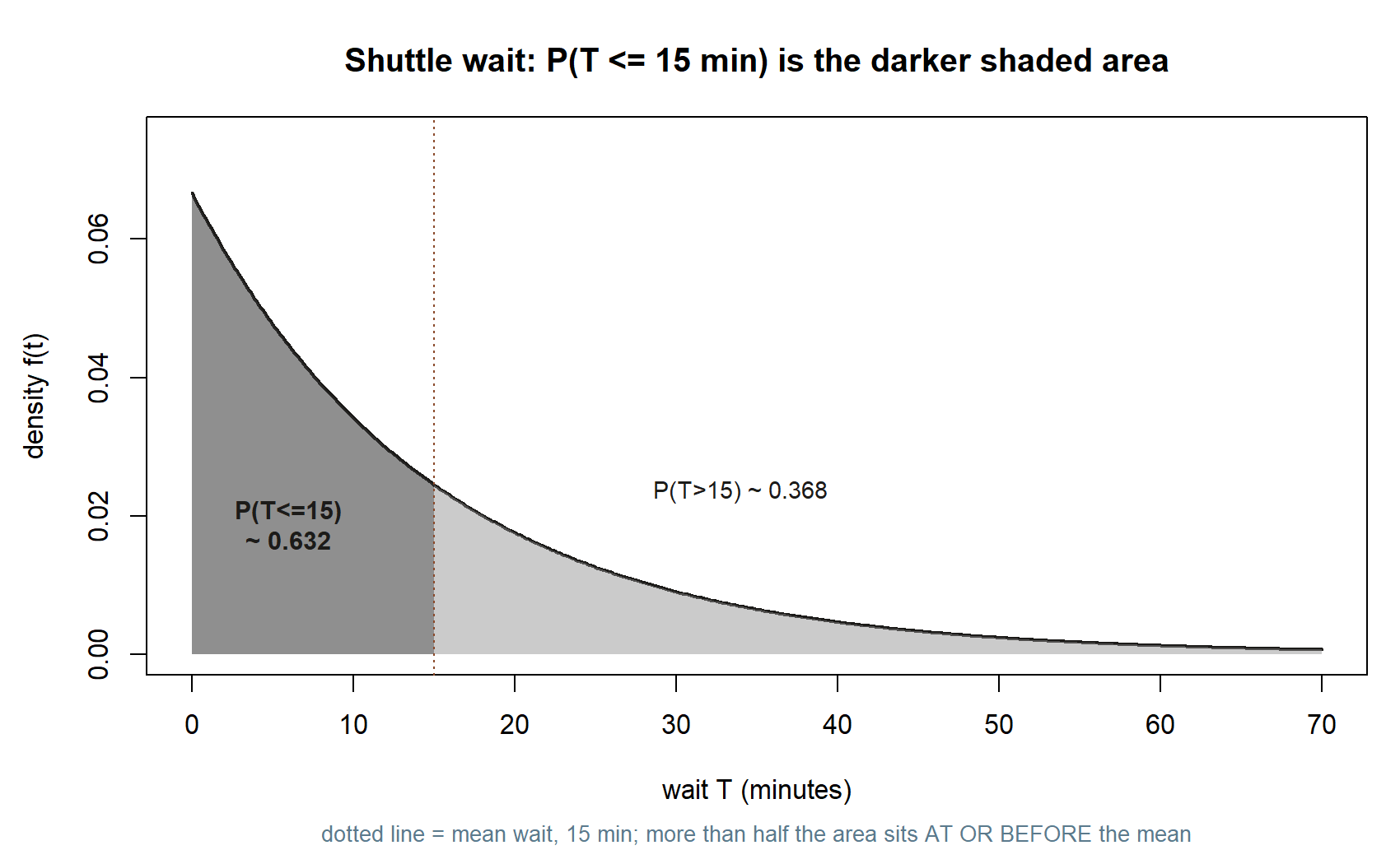
Numeric. What is the chance Maya waits at most 15 minutes for the next shuttle? Fifteen minutes is a quarter of an hour, \(t = 1/4\), so \(\lambda t = 4 \cdot \tfrac{1}{4} = 1\) and

\[ P(T \le 15 \text{ min}) = P\!\left(T \le \tfrac{1}{4}\text{ hr}\right) = 1 - e^{-4 \cdot \frac{1}{4}} = 1 - e^{-1} \approx 0.632. \]

So about \(63.2\%\) of the time the next shuttle comes within one mean-wait, and the other \(36.8\%\) of the time Maya is still waiting after 15 minutes — even though 15 minutes is the average wait. That asymmetry is the signature of the exponential: because the density is highest near zero and trails off to the right, more than half the probability sits below the mean. (Unit care: the rate and the time must share a clock. With \(\lambda\) in events per hour, \(t\) must be in hours, which is why 15 minutes became \(1/4\).)

Figure 2: Seeing the shuttle-wait probability (synthetic). The Exponential(rate \(=4\)/hr) density for the wait \(T\), in minutes, with \(P(T \le 15\text{ min}) \approx 0.632\) shaded darker and the remaining \(P(T > 15\text{ min}) \approx 0.368\) shaded lighter; the dotted line marks the mean wait, 15 minutes.

What the figure shows (non-visual equivalent). The two shaded regions are the two possible outcomes for the next shuttle: arriving within the mean wait of 15 minutes (about 63.2% of the area, darker) or taking longer than that (about 36.8%, lighter). Because the exponential density is tallest at \(t=0\) and decays afterward, more than half the probability sits at or before the mean — the asymmetry named in the numeric work above. Synthetic instructional example; numbers are illustrative.

You can confirm the model by simulation (shown as teaching; not executed in this build):

set.seed(35003)
n_sim <- 100000
# waiting times in hours, rate = 4 per hour
waits <- rexp(n_sim, rate = 4)
mean(waits)              # close to 0.25 hour = 15 minutes
mean(waits <= 0.25)      # close to 0.632

# what running this would show you (a histogram against the theoretical curve):
waits_min <- waits * 60
hist(waits_min, breaks = 80, freq = FALSE, xlim = c(0, 90),
     xlab = "simulated wait (minutes)", main = "Simulated exponential waits")
curve(dexp(x, rate = 4 / 60), add = TRUE, lwd = 2)
abline(v = 15, lty = 3)

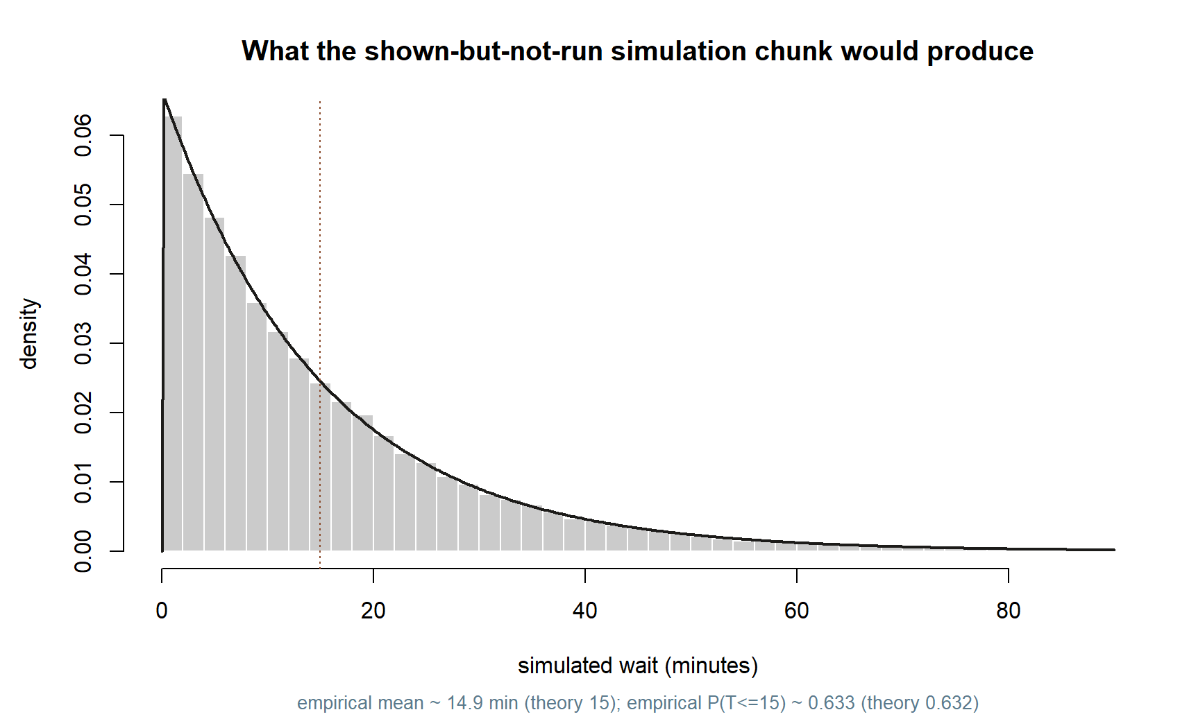
Figure 3: The shown simulation’s expected output (synthetic). A histogram of 100,000 simulated exponential waits — the code above, reproduced exactly (set.seed(35003), rate 4/hr) — with the theoretical density overlaid and the mean wait, 15 minutes, marked.

What the figure shows (non-visual equivalent). This is the picture the code above would produce if you ran it: the simulated histogram tracks the theoretical curve closely, and the simulated mean(waits) and mean(waits <= 0.25) land close to the theoretical 15 minutes and 0.632 computed by hand. The code is shown as a teaching activity and is not executed in this build; this figure shows what running it yourself would produce. Synthetic instructional example; numbers are illustrative.

Worked example — the commute time as a normal (recurring slice)

Maya’s door-to-campus commute is not a count and not a pure waiting time; it is a measurement that piles up around a typical duration, a little longer on bad-traffic days, a little shorter on good ones. Records show it averages 22 minutes with a standard deviation of 5 minutes, roughly symmetric and bell-shaped. Let \(C\) be the commute time in minutes.

Symbolic. A symmetric, bell-shaped measurement is the normal setting. State the parameterization explicitly: \(\mu = 22\) is the mean and \(\sigma = 5\) is the standard deviation (not the variance), so

\[ C \sim \text{Normal}(\mu = 22, \sigma = 5), \qquad E[C] = 22 \text{ min}, \qquad \sigma_C = 5 \text{ min}. \]

To find a probability, standardize: convert \(C\) to a \(z\)-score and use \(\Phi\),

\[ P(C \le c) = \Phi\!\left(\frac{c - \mu}{\sigma}\right) = \Phi\!\left(\frac{c - 22}{5}\right). \]

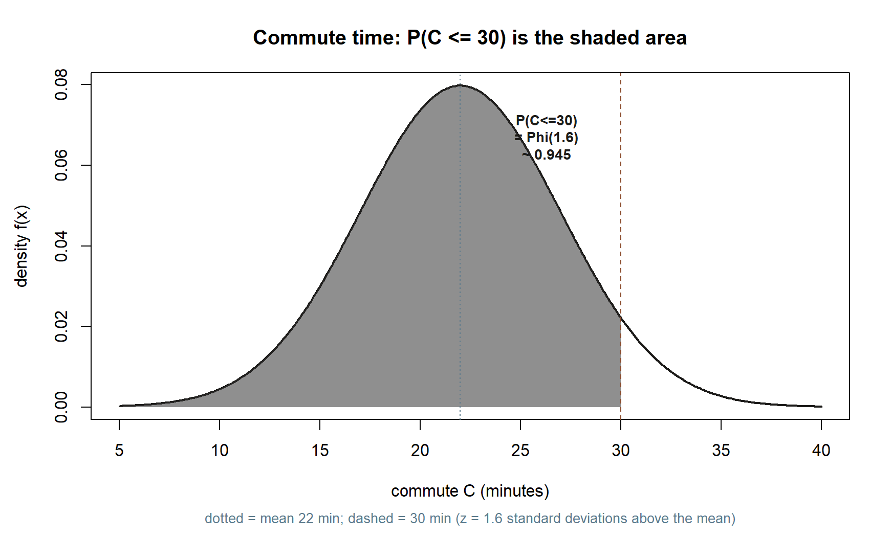
Numeric. Maya wants to arrive within 30 minutes. The \(z\)-score for \(c = 30\) is

\[ z = \frac{30 - 22}{5} = \frac{8}{5} = 1.6, \]

so 30 minutes sits \(1.6\) standard deviations above her average commute, and

\[ P(C \le 30) = \Phi(1.6) \approx 0.945. \]

About \(94.5\%\) of her commutes come in at or under 30 minutes; the other \(5.5\%\) run longer. The whole calculation hinged on reading the second parameter as a standard deviation: treat the \(5\) as a variance and use \(\sigma = \sqrt{5} \approx 2.24\), and the \(z\)-score balloons to about \(3.6\) and the probability to roughly \(0.9998\) — a wildly different, confidently wrong answer from the same formula. This is exactly why the course states the parameterization every time.

Figure 4: Seeing the commute-time probability (synthetic). The Normal(mean \(22\), sd \(5\)) density for the commute \(C\), in minutes, with \(P(C \le 30) = \Phi(1.6) \approx 0.945\) shaded; the dotted line marks the mean, 22 minutes, and the dashed line marks 30 minutes (\(z = 1.6\)).

What the figure shows (non-visual equivalent). The shaded region is every commute of 30 minutes or less — about 94.5% of the bell’s area — bounded on the right by a line exactly \(1.6\) standard deviations above the mean, the \(z\)-score computed above. The unshaded sliver in the right tail, about 5.5% of the area, is every commute that runs longer than 30 minutes. Synthetic instructional example; numbers are illustrative.

Worked example — time to the next customer, and a measurement error (transfer)

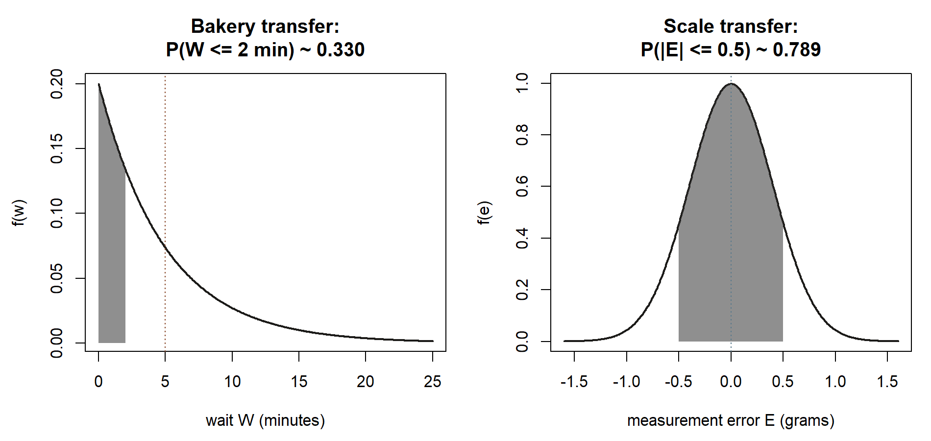
Now move both ideas to brand-new settings to show they are about the structure of the problem, not about Maya. First, an exponential. A small bakery finds customers arrive at a steady, independent average rate of \(\lambda = 12\) per hour during the morning rush. Let \(W\) be the time, in hours, until the next customer walks in. The waiting-time structure gives

\[ W \sim \text{Exponential}(\lambda = 12 \text{ per hour}), \qquad E[W] = \frac{1}{12}\text{ hr} = 5 \text{ minutes}, \]

and the chance the next customer arrives within two minutes (\(t = 2/60 = 1/30\) hour) is

\[ P(W \le 2 \text{ min}) = 1 - e^{-12 \cdot \frac{1}{30}} = 1 - e^{-0.4} \approx 0.330. \]

So even in a brisk rush there is only about a one-in-three chance the next customer appears within two minutes — the same rate-and-reciprocal-mean logic as Maya’s shuttle, in a different store.

Second, a normal. A lab scale used to weigh samples is unbiased but imprecise: repeated weighings of the same object scatter around the true weight with measurement error that is roughly normal, mean \(0\) grams and standard deviation \(\sigma = 0.4\) grams. Let \(E\) be the error on a single weighing. Then

\[ E \sim \text{Normal}(\mu = 0, \sigma = 0.4), \qquad P(|E| \le 0.5) = \Phi\!\left(\frac{0.5}{0.4}\right) - \Phi\!\left(\frac{-0.5}{0.4}\right) = \Phi(1.25) - \Phi(-1.25) \approx 0.789, \]

so a single weighing lands within half a gram of the truth about \(79\%\) of the time. The same normal template fits adult heights, test scores, and any quantity built from many small independent nudges: name the mean, name the standard deviation, standardize, and read \(\Phi\). Synthetic; seed set.

Figure 5: Two transfer contexts, the same shading idea (synthetic). Left: the bakery’s Exponential(rate \(=12\)/hr) wait \(W\), with \(P(W \le 2\text{ min}) \approx 0.330\) shaded. Right: the scale’s Normal(mean \(0\), sd \(0.4\)) measurement error \(E\), with \(P(|E| \le 0.5) \approx 0.789\) shaded (both tails).

What the figure shows (non-visual equivalent). Same shading idea, two new contexts. The bakery panel shades the roughly one-in-three chance the next customer arrives within two minutes; the scale panel shades the roughly four-in-five chance a single weighing lands within half a gram of the truth. Neither picture is about Maya — that is the point of a transfer example: the shape of the argument, shade-the-relevant-area- under-a-named-density, carries over unchanged. Synthetic instructional example; numbers are illustrative.

A common mistake

The classic Week-11 error is a parameterization slip — feeding a number into the wrong slot — and it takes two forms.

The first is the exponential rate-versus-mean swap. Because the mean wait is \(1/\lambda\), it is easy to write the mean into the model as if it were the rate. For Maya’s shuttle the mean wait is 15 minutes and the rate is 4 per hour; set “\(\lambda = 15\)” by mistake and you have made the rate enormous and the mean wait a fraction of a minute. Keep units attached: a rate is events per unit time, a mean is a time, and they are reciprocals — which is also why 15 minutes entered the formula as \(1/4\) hour.

The second is the normal standard-deviation-versus-variance swap. In this course’s \(\text{Normal}(\mu, \sigma)\) the second slot is the standard deviation, but many sources write \(\text{Normal}(\mu, \sigma^2)\) with a variance there. If a problem hands you a variance, take its square root before using it as \(\sigma\); if it hands you a standard deviation, do not square it. For Maya’s commute, \(\sigma = 5\) minutes is the standard deviation, so the \(z\)-score for 30 minutes is \((30 - 22)/5 = 1.6\) — using \(25\) or \(\sqrt 5\) there gives a wrong answer the formula returns without complaint. Whenever you write a continuous model, say the parameterization out loud first; as in Week 9, the arithmetic is almost never the part that goes wrong.

The two slips side by side, using only this week’s own numbers:

Table 1: Two parameterization slips side by side: the exponential rate-vs-mean swap and the normal sd-vs-variance swap, using only this week’s own locked numbers.

Model slot	Correct read	If you swap it	What the swap does
Exponential \(\lambda\) (shuttle wait)	\(\lambda = 4\)/hr is the rate; mean wait \(= 1/\lambda = 15\) min	Set \(\lambda = 15\), treating the mean as if it were the rate	Implied mean wait becomes \(1/15\) hr \(= 4\) min — a wait nearly four times shorter, not the 15 minutes intended
Normal \(\sigma\) (commute time)	\(\sigma = 5\) min is the standard deviation; \(z = (30-22)/5 = 1.6\), \(\Phi(1.6) \approx 0.945\)	Treat \(5\) as a variance, use \(\sigma = \sqrt{5} \approx 2.24\)	\(z\) balloons to about \(3.6\), \(\Phi(3.6) \approx 0.9998\) — a confidently wrong, near-certain answer

Both rows plug the same locked numbers into the same formula; only the parameter slot changes, and the formula never complains either way — which is exactly why saying the parameterization out loud first is the habit that catches the error before the arithmetic does.

Low-stakes self-checks (ungraded)

These are for your own practice — nothing here is collected or graded.

1. A bus is scheduled for 8:00 but actually shows up at a time spread uniformly between 8:00 and 8:10. Name the model and its parameters, then find the probability it arrives in the first four minutes.
2. For Maya’s shuttle, \(T \sim \text{Exponential}(\lambda = 4/\text{hr})\). Explain in one sentence why the mean wait is 15 minutes rather than 4, and confirm that \(P(T \le 15\text{ min}) = 1 - e^{-1}\) by checking that \(\lambda t = 1\) when \(t = 1/4\) hour.
3. Calls reach a help desk at a steady, independent rate of \(\lambda = 6\) per hour. State the model for the wait until the next call, give its mean wait in minutes, and write the expression for the probability the next call comes within five minutes (you do not need to evaluate it).
4. For Maya’s commute, \(C \sim \text{Normal}(22, 5)\) minutes. Compute the \(z\)-score for a 27-minute commute, and say in words what that \(z\)-score means before you look up any area.
5. Without computing a final number, decide which model fits each and name its parameter(s): (a) the exact spot a raindrop lands along a 10-cm pencil left in the rain; (b) the time between independent text messages arriving on a busy afternoon; (c) the heights of adult women in a large population. Justify each by the assumption that makes it fit, and for the last one state which slot is the standard deviation.

Reading and source pointer

For the continuous-model definitions and their densities, read Grinstead & Snell, Chapter 5 — Important Distributions (continuous part), which develops the uniform, exponential, and normal families and their basic properties: https://www.dartmouth.edu/~chance/teaching_aids/books_articles/probability_book/book.html.

This week also draws on the secondary course text. See MIT OpenCourseWare 18.05 for its treatment of continuous random variables and, in particular, the normal distribution and standardizing — a useful second pass on turning a normal question into a standard-normal area with \(\Phi\): https://ocw.mit.edu/courses/18-05-introduction-to-probability-and-statistics-spring-2022/.

These notes are the course’s own synthesis, grounded in but not copied from the sources.

Public vs. graded

These notes, the examples, and the practice here are public and ungraded — study material only. No graded prompts, answer keys, rubrics, point values, or due dates appear on this site. Graded checkpoints, quizzes, homework, labs, the midterm, the project, and the final live in Blackboard (the LMS), which is authoritative for due dates, submissions, and grades. If this page and Blackboard ever disagree, follow Blackboard.

Looking ahead

You now have the two big families — discrete models (Week 9) and continuous models (this week) — and the machinery to read a probability off either. So far every example has involved one random variable at a time. Next week we let variables interact: joint distributions and dependence, where two random quantities live together and we measure how strongly one moves with the other through covariance and correlation. Maya’s thread carries us straight in: whether it rains and whether her shuttle is late are not independent (you saw that back in Weeks 3–4), and Week 12 quantifies that link. After that, Week 13 returns to the normal one more time — when we add or average many random variables, the normal reappears as a limit, which is the central limit theorem.

See also

• Notation glossary — the binding symbols and the model parameterizations (\(\text{Exponential}(\lambda)\) as a rate with mean \(1/\lambda\); \(\text{Normal}(\mu, \sigma)\) as mean and standard deviation).
• Distribution reference — a one-stop table of each model’s density, mean, standard deviation, support, and the R *unif/*exp/*norm functions (including that rexp takes a rate and rnorm takes mean and sd).
• Week 10 — Continuous random variables — where density, area as probability, and the cdf \(F(x) = P(X \le x)\) were first built.
• Week 9 — Common discrete models — the discrete partner to this week, and where the Poisson arrival rate \(\lambda = 4\) per hour first appeared.
• Week 12 — Joint distributions and dependence — the next step, where two random variables interact.
• Course syllabus — overall structure, schedule, and where graded work lives.