Week 14 — Inference project workshop

Putting two inferential methods to work on one question of your own

A framing note before anything else: this week introduces no new inferential machinery. Every tool the project needs — estimation, standard errors, confidence intervals, hypothesis tests, bootstrap resampling, permutation tests, Bayesian updating — was built in Weeks 1 through 13. This week is workshop time: guidance for applying what you already have to a question of your own choosing. Nothing below assigns a grade, a rubric, or a due date; those live in Blackboard (see Public vs. graded).

The week question

You already know how to run a confidence interval, a hypothesis test, a bootstrap, a permutation test, and a Bayesian update, one at a time, on data the course handed you. The project asks a harder question: given a question you choose, how do you pick two genuinely different inferential methods that both speak to it, run both honestly, and say something responsible about what you learned, including where the two methods agree, where they differ, and why?

Why this matters

Real inferential work rarely arrives labeled “use a two-sample t-test here” or “this is a bootstrap problem.” It arrives as a question about the world, and the analyst decides which tools apply, what each leans on, and how much to trust the answer any one tool gives. Comparing two methods on the same question, rather than running one and reporting its output as the only possible answer, is the single best habit this course can leave you with: it forces you to notice which conclusions are robust across reasonable analytical choices and which are artifacts of one method’s assumptions. That is exactly what the final-third project asks you to do.

Learning goals

By the end of this week you should be able to:

State a project question in inferential terms: a population, a parameter of interest, and the kind of claim (estimation, comparison, or evidence-for-a-hypothesis) the question is really asking for.
Choose two methods that are genuinely different — differing in framework (frequentist vs. Bayesian), mechanism (formula-based vs. resampling-based), or assumption structure — not two cosmetically different versions of the same idea.
Build a short checklist for comparing what each method assumes, and use it to identify where two methods’ assumptions overlap and diverge.
Draft a responsible, assumption-aware interpretation reporting what both methods conclude, where they agree or disagree, without overclaiming certainty either method does not actually provide.
Recognize the Week 13 MAC Study comparison as a worked model of this kind of multi-method project.

Core vocabulary

Inferential question: a question naming a population, an unknown parameter (a mean, a proportion, a difference, a rate), and the kind of conclusion sought. “Do MAC visits average more than 45 minutes?” is inferential; “what do students think about the MAC?” is not, until narrowed to a specific parameter and claim.
Method family: one of the four inferential approaches this course has built — classical/frequentist, simulation-based/resampling (bootstrap, permutation), likelihood-based (MLE), and Bayesian. A genuinely different second method usually comes from a different family, not a different formula within one.
Assumption structure: the conditions a method leans on to be valid — independence, a distributional shape, a known or estimated standard error, exchangeability under a null, or a prior distribution. Two methods can reach similar conclusions while resting on different assumption structures.
Convergence and divergence: when two methods reach compatible conclusions (as in Week 11’s permutation p-value tracking its normal-approximation cross-check), that is reassuring but not proof of anything beyond “these assumptions happen to agree here.” Divergence is information about which assumptions are doing the work, not a failure.
Responsible interpretation: a written conclusion stating what each method found in that method’s own terms (a CI is not “a probability,” a p-value is not “the probability the null is true”), flagging any assumption the analysis depends on that the data cannot fully verify.

Concept development

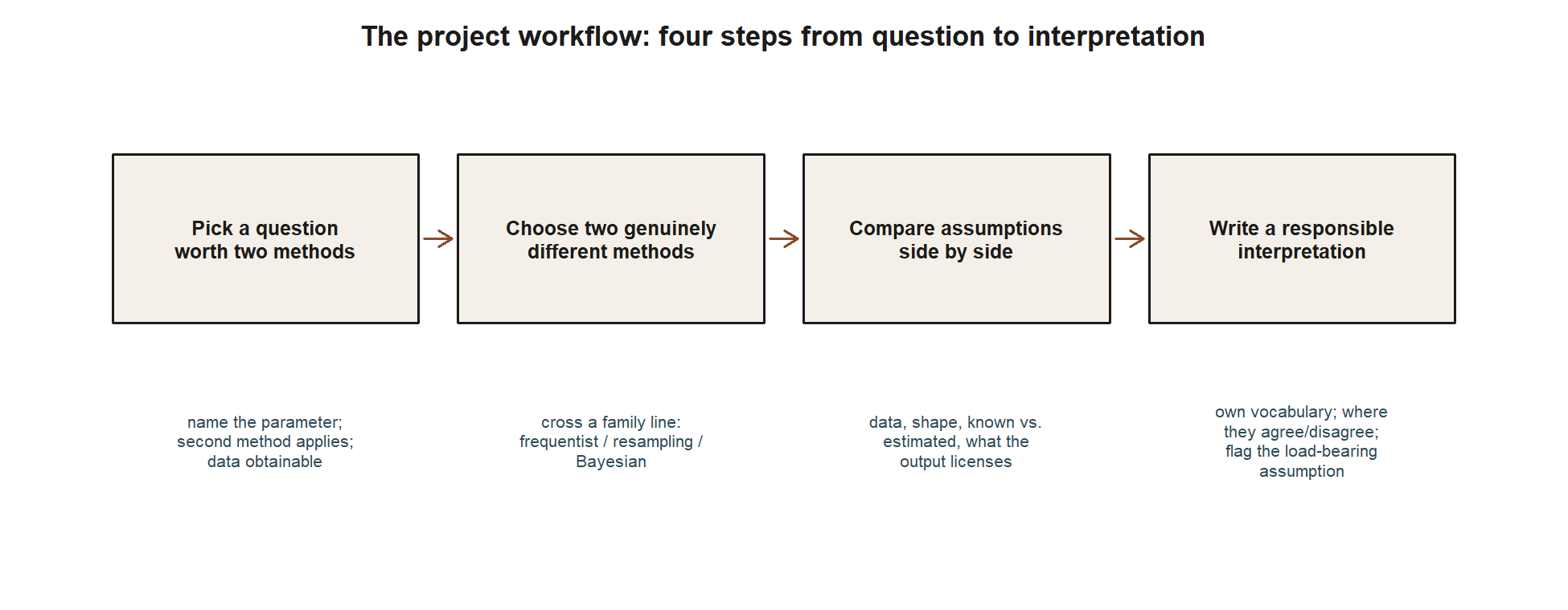
Every stage of this workshop — and both worked examples below — walks the same four-step path. Keep this picture in mind as the anchor for everything that follows.

A left-to-right flow diagram of four boxes connected by arrows: Pick a question worth two methods, Choose two genuinely different methods, Compare assumptions side by side, Write a responsible interpretation. A short subtext line under each box names what that step checks. — Figure 1: **The project workflow: four steps from question to interpretation.** Every project this week supports follows the same path: pick a question worth two methods, choose two genuinely different methods, compare their assumptions side by side, and write a responsible, assumption-aware interpretation. Both worked examples below walk this exact four-step path.

What the figure shows (non-visual equivalent). The workshop’s four steps, in order: (1) name the parameter and confirm a second method applies and the data are obtainable; (2) choose two methods that cross a family line — frequentist vs. resampling, frequentist vs. Bayesian, or a standard test vs. a permutation test; (3) compare what each method assumes about data collection, distributional shape, known-vs-estimated quantities, and what its output licenses; (4) write an interpretation in each method’s own vocabulary, naming where the two agree or disagree and which assumption is most load-bearing.

Picking a question worth two methods

A good project question is narrow enough to answer with the data you can actually get, but substantive enough that a reader would care about the answer. Three checks help. First, can you name the parameter? If you cannot write down, in one phrase, what unknown population quantity your question is about, the question is still a topic, not yet an inferential question — “are online reviews mostly positive?” becomes inferential once it becomes “what proportion of all reviews are 4 or 5 stars?” Second, does more than one method actually apply? Some questions are naturally suited to comparison — a proportion estimated two ways (formula-based CI vs. bootstrap CI), a group comparison tested two ways (a two-sample test vs. a permutation test), or a parameter analyzed both frequentist and Bayesian. If you cannot see a second reasonable method before you start, the question is likely too narrow. Third, is the data realistically obtainable? A project works best on data you can collect, simulate honestly, or responsibly source (with provenance stated), at a scale that makes both chosen methods meaningful.

A question phrased as estimation pairs naturally with a formula-based CI and a bootstrap CI, or a frequentist CI and a Bayesian credible interval. A question phrased as a comparison pairs naturally with a two-sample test and a permutation test.

Choosing two genuinely different methods

The project asks for at least two inferential methods that speak to the same question — not two unrelated analyses, and not two versions of the same idea wearing different notation. A useful test: if switching methods mainly changes which formula you type and nothing about what you had to assume to get there, the two are not different enough. Genuine difference usually comes from crossing one of three lines.

Frequentist vs. resampling-based: a formula-based confidence interval (Week 7) alongside a percentile bootstrap interval (Week 10) for the same parameter — the formula-based interval appeals to a Normal sampling distribution, the bootstrap resamples the data itself, and Week 10’s bootstrap CI landed close to Week 7’s formula-based CI for the MAC visit-duration mean. Frequentist vs. Bayesian: a confidence interval or p-value (Weeks 7 to 9) alongside a Bayesian posterior interval (Week 12) — these differ in what the interval even means, a frequentist CI a property of the procedure across repeated sampling, a Bayesian credible interval a direct probability statement given prior and data. A standard two-sample test vs. a permutation test: a normal-approximation statistic and p-value (Week 8) alongside a permutation p-value (Week 11) built by reshuffling group labels — Week 11’s workshop-vs-control comparison shows how close these can land when both sets of assumptions hold reasonably well.

Whichever pairing you choose, write down before you compute anything which two methods you plan to use and why they differ enough to be worth comparing.

The same branching shows up as a picture before it shows up as a table: start from your question’s shape, follow the branch that matches, and land on a method pairing.

A decision tree. The root box reads what shape is your question. It branches into two boxes: estimating one parameter, and comparing two groups. Estimating one parameter branches into two leaf boxes: formula-based CI week 7 versus bootstrap CI week 10, and frequentist CI or test weeks 7 through 9 versus Bayesian credible interval week 12. Comparing two groups branches into one leaf box: two-sample z-test week 8 versus permutation test week 11. A short check question sits below each leaf box. — Figure 2: **Method selection: from question shape to a method pairing.** The same decision the table below spells out, drawn as a tree: an estimation question branches toward a formula-vs-bootstrap pairing or a frequentist-vs-Bayesian pairing; a group-comparison question branches toward a z-test-vs-permutation-test pairing.

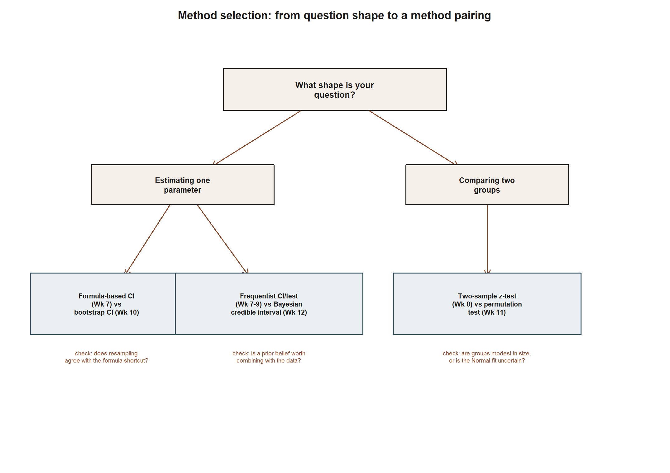
Table — a method-selection matrix. Use this as a checklist while you pick your own pairing — the numeric companion to the tree above: find the row whose “question shape” matches your project, then read across for the two methods and the rule of thumb on when that pairing is worth running.

Question shape	Method 1	Method 2	Genuinely different because…	Good fit when…
Estimating one parameter	Formula-based CI (Week 7)	Percentile bootstrap CI (Week 10)	one leans on a Normal sampling-distribution formula, the other resamples the data directly	you want to check whether a normal-theory shortcut and a resampling approach agree
Estimating one parameter	Frequentist CI or test (Weeks 7–9)	Bayesian credible interval (Week 12)	they answer different questions — long-run procedure behavior vs. a direct probability statement about the parameter	you have (or are willing to state) a prior belief worth combining with the data
Comparing two groups	Two-sample \(z\)-test (Week 8, extended)	Permutation test (Week 11)	one assumes a Normal approximation is valid; the other only assumes exchangeable labels under the null	your two groups are modest in size or you are unsure the Normal approximation applies cleanly

Every row above is a genuinely different family crossing (frequentist vs. resampling, frequentist vs. Bayesian, formula-based vs. relabeling-based) — not two cosmetically different formulas from the same family, which is exactly the shortcut the common-mistake section below warns against.

A checklist for comparing assumptions

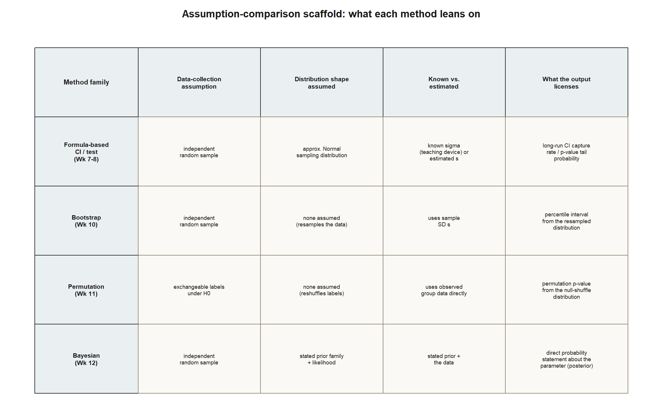
Once you have chosen two methods, work through the same short checklist for each, side by side: what does it assume about how the data were collected (independence, a sampling design, exchangeable labels under a null)? What does it assume about the shape of the sampling distribution, if anything (approximately Normal for a formula-based CI or test; no shape assumed for a bootstrap or permutation test; a specific prior family for a Bayesian analysis)? What does it treat as known versus estimated (a known-σ simplification versus an estimated s; a stated prior versus none)? What kind of statement does its output license (a CI is a claim about the long-run behavior of the procedure, not a probability about one interval; a p-value is a claim about how surprising the data are under H₀, not a probability that H₀ is true; a Bayesian posterior interval is a direct probability statement about the parameter)? And where would it break down?

Filling in this checklist for both methods is what lets you write the comparison honestly, instead of running two procedures and reporting two numbers with no discussion of why they might, or might not, agree.

Laid out side by side, the checklist looks like this for the four method families this course has built:

A five-by-five grid. Row headers name four method families: formula-based CI or test week 7 to 8, bootstrap week 10, permutation week 11, and Bayesian week 12. Column headers name four questions: data-collection assumption, distribution shape assumed, known versus estimated, and what the output licenses. Each cell holds a short phrase answering that question for that method family. — Figure 3: **Assumption-comparison scaffold: what each method leans on.** The same checklist questions — a data-collection assumption, a distributional-shape assumption, what is known versus estimated, and what the output licenses — answered for each of the four method families covered this semester.

What the figure shows (non-visual equivalent). All four method families assume an independent sample except permutation, which instead assumes exchangeable labels under the null. Formula-based and Bayesian methods assume a distributional shape (Normal, or a stated prior family); bootstrap and permutation assume none, working directly from resampled or reshuffled data. Each family licenses a different kind of output statement: a long-run capture rate or tail probability for the two frequentist rows, a resampled interval for bootstrap, a null-shuffle p-value for permutation, and a direct probability statement about the parameter for Bayesian.

Writing a responsible, assumption-aware interpretation

The last and most important step is translating two sets of computed numbers into a written conclusion a reader can trust. Three habits separate a responsible interpretation from an overclaiming one. First, state each method’s conclusion in that method’s own vocabulary — do not describe a frequentist CI as “a 95% chance the true parameter is in this range” (Week 7’s convention-risk flag), and do not describe a Bayesian posterior interval using frequentist p-value language. Second, name where the two methods agree and where they do not, and say why: near-coincidence between, say, a formula-based CI and a bootstrap CI is reassuring precisely because the two rest on different assumptions that happen to both be satisfied here; disagreement calls for discussing which method’s assumptions are more plausible for your data, not for preferring whichever supports your hypothesis. Third, flag the assumption most load-bearing for your conclusion, explicitly — every method rests on at least one assumption you cannot fully verify from the data alone; name it rather than hide it.

None of this requires certainty. A responsible interpretation may conclude “the two methods broadly agree, and here is why I trust that agreement” or “they disagree here, most likely because of [a stated assumption], and here is what I would check next” — both are honest, complete answers.

Worked examples

Worked example — The MAC Study: what a good project looks like

This example walks the four-step workflow pictured above end to end, and lands on the method-selection diagram’s frequentist-vs-Bayesian branch.

Week 13 built exactly this kind of comparison for the MAC Study’s usage-rate question, worth revisiting here as a model, not as new material. The question was: what is the true usage rate π, the proportion of students who use the MAC at least once in a given week? Week 13 laid the classical/frequentist confidence interval and the Bayesian posterior side by side, both built from the same n = 100, k = 38 survey (p̂ = 0.38), with the Beta(3, 7) prior from Week 12 supplying the Bayesian piece.

Notice what made that a strong comparison, because it is the template for your own project. The question was named precisely (estimate π) before any method was chosen. The methods were genuinely different in kind — a frequentist CI leaning on a Normal-approximation standard error, and a Bayesian posterior leaning on a stated prior — not variations on one formula. The comparison stated where the methods agreed and why: the frequentist CI (0.285, 0.475) and the Bayesian 95% credible interval (0.283, 0.463) land close to each other, attributed to the prior being comparatively weak (Beta(3, 7), a prior sample size of only 10) relative to the n = 100 data, so the data dominate the posterior and pull the Bayesian answer close to the frequentist one. Each method’s output was reported in its own vocabulary: the CI was never described as “a 95% probability” claim, while the posterior interval was described as a direct probability statement about π, because that is what a Bayesian credible interval actually licenses.

Your project will not be about the MAC Study — it should be about a question of your own — but this shape (name the parameter, choose genuinely different methods, compare assumptions explicitly, report each method in its own vocabulary, say where and why they agree or disagree) is the shape a strong project takes, whatever the topic.

Worked example — Transfer: sketching a project plan (synthetic)

This sketch follows the same four-step workflow pictured above, landing on the method-selection diagram’s group-comparison branch — deliberately without computing anything yet.

The following question and numbers are synthetic, invented to illustrate project planning only — not drawn from the MAC Study and not a completed analysis.

Suppose a student proposes this question: “Among students at a large public university, is usage of a library-based tutoring service higher among first-year students than among upperclassmen?” The parameter is a difference in usage proportions, π₁ − π₂. Method one is a two-proportion z-test (Week 8’s logic extended to two groups). Method two, genuinely different, is a permutation test (Week 11’s logic) that reshuffles the first-year/upperclassman labels to build a null distribution directly from the data, with no Normal-approximation formula. The assumption checklist, sketched in advance: the z-test needs a large-enough sample for the Normal approximation; the permutation test needs only that labels are exchangeable under the null, a milder assumption, but one still requiring the two groups to have been sampled comparably (not, say, one online and one in person). A responsible interpretation would report whether the two agree or disagree, and why.

This sketch is left deliberately incomplete — no data collected, no numbers computed — because the point is the planning move itself, which transfers directly to whatever question your own project asks.

A common mistake

Treating “two methods” as two cosmetically different formulas instead of two different assumption structures. A common shortcut is to run a hypothesis test twice with two slightly different formulas (say, a z-test and a nearly identical t-test) and call that “comparing two methods.” Both lean on essentially the same Normal-approximation logic and assumptions, so the comparison mostly tests whether two similar formulas give similar answers — which they almost always will, and which does not teach a reader much. Choose a second method from a genuinely different family instead (resampling-based instead of formula-based, or Bayesian instead of frequentist), so the comparison tests whether a different set of assumptions leads to a different or similar conclusion.

Low-stakes self-checks (ungraded)

Write a project question as a single sentence naming the population, the parameter, and the kind of claim (estimate or test) you are after. If you cannot, the question likely needs narrowing.
For your chosen question, name two candidate methods and explain what each assumes that the other does not.
Revisit the Week 13 MAC Study comparison and state, in your own words, why the frequentist CI and the Bayesian credible interval for π landed close together.
In the synthetic library-tutoring sketch, suppose the z-test and the permutation test for π₁ − π₂ gave noticeably different p-values. List two explanations rooted in the assumption checklist above.
Draft what a responsible interpretation would say if your two methods agreed closely, and a separate draft of what it would say if they did not.

Reading and source pointer

This week points back to MIT OCW 18.05 as review support rather than new material: the sampling-distribution, estimation, testing, bootstrap, and Bayesian-inference sections already used in Weeks 2 through 13 are the right places to revisit if a method you are choosing needs a refresher. No new chapter or topic is introduced this week. These notes are the course’s own synthesis, grounded in but not copied from the sources.

Public vs. graded

These notes, the examples, and the practice here are public and ungraded — study material only. No graded prompts, answer keys, rubrics, point values, or due dates appear on this site. Graded inference checkpoints, quizzes, homework, labs, the midterm, the project, and the final live in Blackboard (the LMS), which is authoritative for due dates, submissions, and grades. If this page and Blackboard ever disagree, follow Blackboard.

Looking ahead

Week 15 closes the course with a one-day final synthesis (last class Monday, Dec 7), pulling the whole MAC Study thread into a single picture. The project-planning habits from this week — naming a parameter, choosing genuinely different methods, comparing assumptions explicitly, writing a responsible interpretation — are the same habits final synthesis, and the cumulative final exam (Dec 9 to 15 window), draw on as well.