Week 3 — Estimators and standard errors

How much does an estimate wobble from sample to sample?

The week question

You have one sample. From it you compute one number — a sample mean, a sample proportion, whatever the question calls for. That number is your best guess at some unknown population quantity. But if you had drawn a different sample from the same population, you would have gotten a different number. How do you describe, honestly and quantitatively, how much that number would have wobbled? This week answers that question by introducing the standard error, and by drawing a line — one you will need for the rest of the course — between the standard error of an estimator and the standard deviation of the data you actually collected.

Why this matters

Every confidence interval you build starting in Week 7, every hypothesis test starting in Week 8, and every bootstrap or Bayesian calculation later in the course leans on a standard error. If you cannot correctly state what a standard error is a standard error of, you cannot correctly interpret any of the machinery built on top of it. This week is short — Labor Day trims a class meeting off it — but it is not optional: it is the hinge between “here is a single number I computed” (Week 1) and “here is how uncertain that number is” (Weeks 7 onward).

Learning goals

By the end of this week you should be able to:

• Define an estimator as a function of sample data used to produce a guess at an unknown parameter, and distinguish an estimator (the rule) from an estimate (the number it produces on one particular sample).
• Define the standard error of an estimator and explain, in words, what “sampling variability” means.
• State clearly why the standard error and the sample standard deviation are not the same quantity, even though they are computed from related ingredients.
• Compute \(SE(\bar{x})\) for a sample mean under a known population SD, and \(SE(\hat{p})\) for a sample proportion.
• Read a standard error correctly: as a description of how much an estimator would vary across repeated samples, not as a description of any single data point.

Core vocabulary

• Estimator (\(\hat{\theta}\)): a rule, applied to sample data, that produces a guess at an unknown parameter \(\theta\). The sample mean \(\bar{x}\) is an estimator of the population mean \(\mu\); the sample proportion \(\hat{p}\) is an estimator of the population proportion \(\pi\).
• Estimate: the specific numeric value an estimator takes on for one particular sample. \(\bar{x} = 49.8\) is an estimate; “\(\bar{x}\)” the formula is the estimator.
• Sampling variability: the fact that an estimator’s value changes from sample to sample, purely because different samples contain different observations — even when every sample is drawn the same way from the same population.
• Standard error, \(SE(\hat{\theta})\): the standard deviation of the estimator’s own sampling distribution — a theoretical description of how much \(\hat{\theta}\) would vary if you repeated the sampling process over and over. It is a property of the estimator and the sampling design, not of any one sample.
• Sample standard deviation, \(s\) (or the known \(\sigma\) in a known-SD teaching setup): a description of how spread out the individual observations are within the one sample you collected (or within the population, for \(\sigma\)). It answers “how variable are individual data points?”, not “how variable is my summary estimate?”.

Concept development

An estimator is a rule, not a number

Start from Week 1’s setup: a population has an unknown parameter (a mean \(\mu\), a proportion \(\pi\)), and you want to learn about it from a sample. An estimator is the recipe you apply to whatever sample you happen to draw. For the population mean, the natural estimator is the sample mean: \[\hat{\mu} = \bar{x} = \frac{1}{n}\sum_{i=1}^{n} x_i.\] For the population proportion, the natural estimator is the sample proportion: \[\hat{\pi} = \hat{p} = \frac{k}{n},\] where \(k\) is the count of “successes” in a sample of size \(n\).

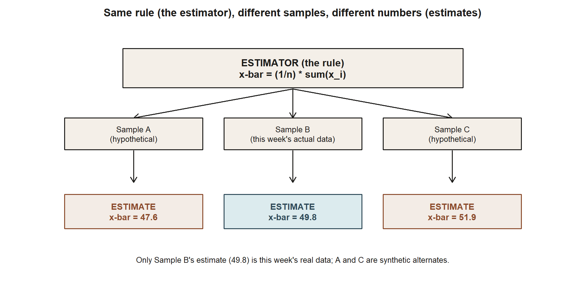
Notice that \(\bar{x}\) and \(\hat{p}\) are formulas — they take a sample as input and return a number as output. Before you draw the sample, the estimator is a random variable: it could come out any number of ways, depending on which observations happen to land in your sample. After you draw the sample and plug in the actual numbers, you get one estimate — a fixed number, no longer random. Keeping “estimator” (the rule, random, capital-letter thinking) and “estimate” (the resulting number, fixed, one sample) distinct is the first habit this week asks you to build.

Figure 1: An estimator is a rule; an estimate is the one number it produces on a particular sample (synthetic). The same formula \(\bar{x} = (1/n)\sum x_i\) applied to three different hypothetical samples produces three different numbers — only the middle one, 49.8, is this week’s actual MAC Study estimate; the other two are synthetic alternates shown to make the rule-versus-number distinction concrete.

Sampling variability, in one picture (traced back to Week 2)

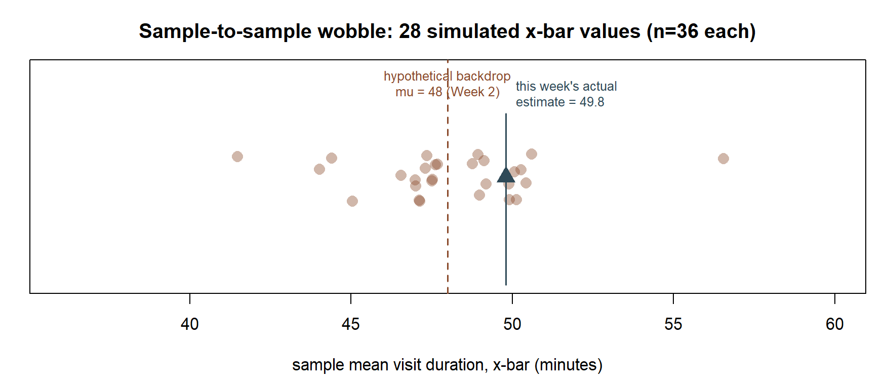
Week 2 built the idea of a sampling distribution by simulation: draw a sample, compute \(\bar{x}\); draw another sample of the same size from the same population, compute \(\bar{x}\) again; repeat many times. The resulting collection of \(\bar{x}\) values is not all the same number — it forms its own distribution, the sampling distribution of \(\bar{x}\), centered near the true \(\mu\) but spread out around it. That spread is what a standard error is built to measure.

The key conceptual move this week makes is turning that simulated picture into a single summary number: the standard deviation of the sampling distribution itself. That number is the standard error. You do not need to actually resimulate a sampling distribution every time you want a standard error — for many familiar estimators, probability theory gives you a formula for \(SE(\hat{\theta})\) directly, without simulation. The next subsection derives the two formulas you will use constantly for the rest of the term.

Figure 2: Sample-to-sample wobble (synthetic): the same recipe, run 28 times, gives 28 different numbers. Each dot is the sample mean \(\bar{x}\) from one simulated 36-visit sample drawn from Week 2’s stipulated hypothetical backdrop, Normal(\(\mu=48\), \(\sigma=15\)) — a teaching device, not a known fact. The dots scatter around 48 rather than landing on it exactly; this week’s actual estimate, \(\bar{x}=49.8\), is one further draw from the same process, marked separately.

What the figure shows (non-visual equivalent). If the MAC visit-duration sampling process were repeated many times under the hypothetical backdrop Normal(\(\mu=48\), \(\sigma=15\)), the resulting sample means would not all equal 48 — they would scatter around it, sample to sample. This week’s actual estimate, \(\bar{x}=49.8\), is exactly this kind of draw: one specific outcome of a process that could have landed elsewhere. That scatter is precisely what a standard error is built to measure. Synthetic instructional example; numbers are illustrative.

Two standard-error formulas you will use constantly

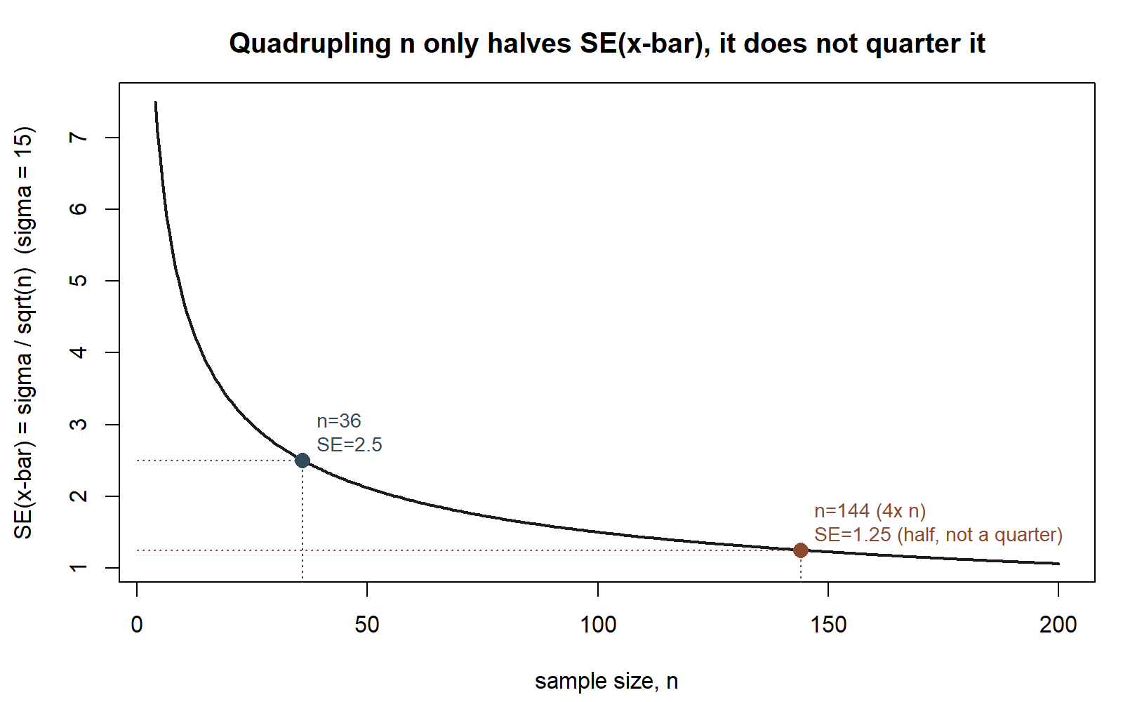
Standard error of a sample mean, known \(\sigma\). If individual observations have population standard deviation \(\sigma\), and you average \(n\) of them, the standard error of the sample mean is \[SE(\bar{x}) = \frac{\sigma}{\sqrt{n}}.\] This says two things worth sitting with. First, larger samples produce less variable estimates — the \(\sqrt{n}\) in the denominator means quadrupling your sample size only cuts the standard error in half, not to a quarter, a fact worth remembering when you plan a study. Second, the standard error scales directly with how variable individual observations already are (\(\sigma\)): noisier raw data means a noisier mean, all else equal.

Figure 3: SE(\(\bar{x}\)) shrinks with \(\sqrt{n}\), not with \(n\) (synthetic curve traced from the formula above). Quadrupling the sample size from 36 to 144 only cuts SE(\(\bar{x}\)) in half (2.5 to 1.25), not to a quarter — a direct picture of the \(\sqrt{n}\) claim made just above.

Standard error of a sample proportion. If you are estimating a proportion \(\pi\) from a sample of size \(n\) with sample proportion \(\hat{p}\), the standard error is \[SE(\hat{p}) = \sqrt{\frac{\hat{p}(1-\hat{p})}{n}}.\] Here \(\hat{p}(1-\hat{p})\) stands in for a “variance-like” quantity: it is largest when \(\hat{p}\) is near 0.5 (most uncertain about which way an individual observation goes) and shrinks toward 0 as \(\hat{p}\) approaches 0 or 1 (almost everyone or almost no one has the trait, so an individual observation is nearly predictable). Notice this formula uses the estimated \(\hat{p}\) in place of an unknown true \(\pi\) — a small but important practical compromise you will see named again in later weeks: since the true \(\pi\) is unknown (that is the whole point of estimating it), you plug in your best available substitute, \(\hat{p}\), to get a usable number.

The distinction that trips almost everyone up: SE vs. sample SD

This is the concept this compressed week most needs you to walk away with, precisely because the two quantities share ingredients and look similar on the page.

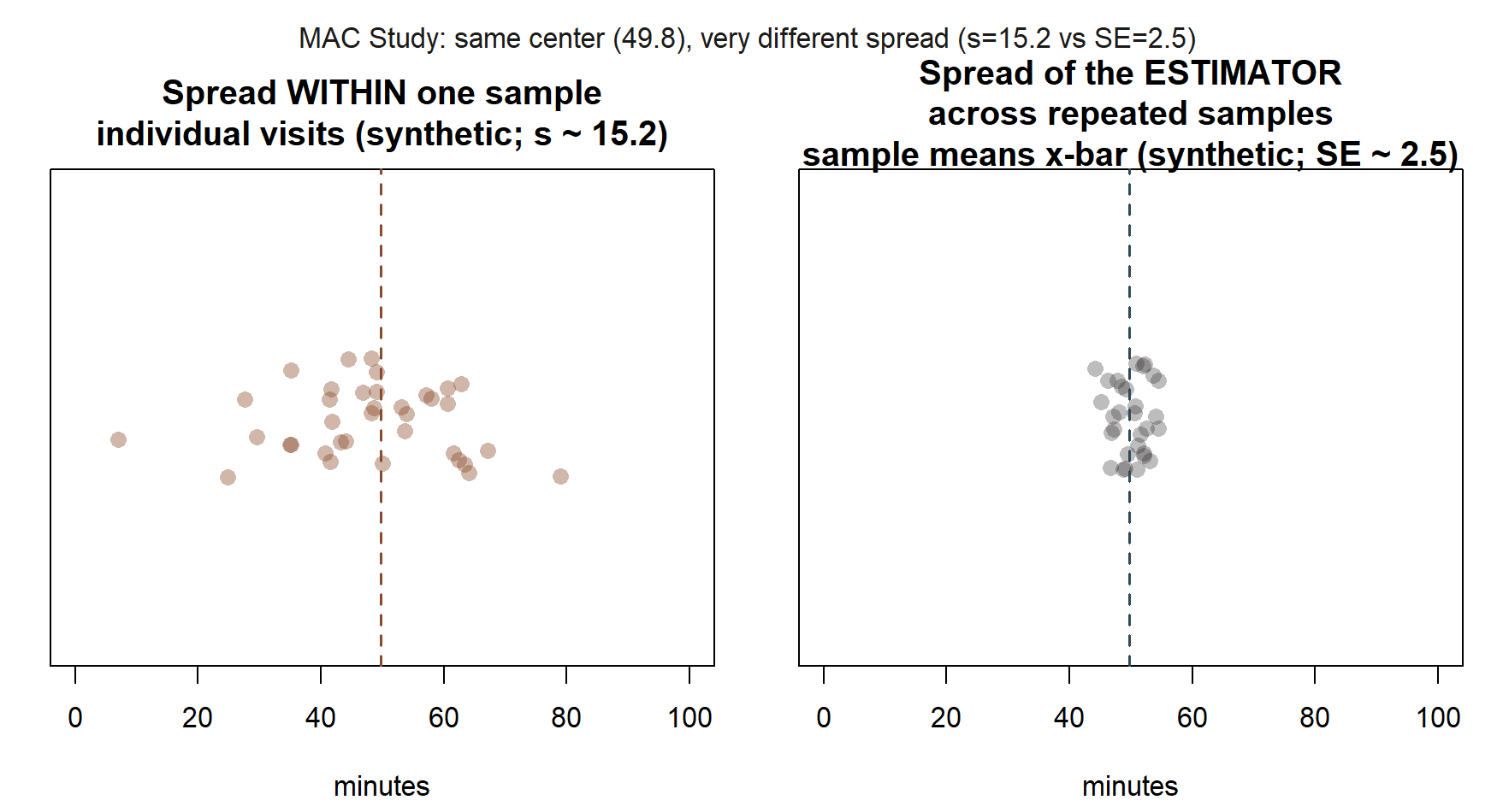
• The sample standard deviation \(s\) describes spread within your one dataset: how far a typical individual observation sits from the sample mean. It answers, “if I picked one MAC visit at random from my 36, how far from 49.8 minutes would I expect it to be?”
• The standard error \(SE(\bar{x})\) describes spread across hypothetical repeated samples of the summary statistic itself: how far a typical sample mean, computed from a fresh sample of the same size, would sit from the true population mean. It answers, “if I redid this whole 36-visit study many times, how much would my computed \(\bar{x}\) bounce around?”

The formula \(SE(\bar{x}) = \sigma/\sqrt{n}\) makes the relationship explicit: the standard error is the data-level standard deviation shrunk by \(\sqrt{n}\), because averaging cancels out some of the individual noise. A standard error is therefore always a statement about an estimator’s variability, never a restatement of how spread out the raw data are. Confusing the two — reporting \(s\) where a reader expects \(SE(\bar{x})\), or vice versa — is common enough that it gets its own section below.

Table 1. Four terms that are easy to blur, MAC Study instance. Read down the “what it describes” column first — that column is the whole distinction this week is built to teach. The last two rows are drawn as pictures, not just formulas, in the spread-comparison figures inside the worked examples below.

Term	What it describes	Varies with \(n\)?	MAC Study value
Estimator	a rule/formula, applied to any sample of the right kind	not a number — a procedure	“take the sample mean,” “take \(k/n\)”
Estimate	the one number that rule produces on this sample	fixed once the sample is drawn	\(\bar{x} = 49.8\); \(\hat{p} = 0.38\)
Sample SD (\(s\)/\(\sigma\))	spread of individual observations within one sample/population	shrinks only slowly, reflects raw data spread	\(\sigma \approx 15\) minutes
Standard error	spread of the estimator itself across hypothetical repeated samples	shrinks with \(\sqrt{n}\)	\(SE(\bar{x}) = 15/\sqrt{36} = 2.5\) minutes

The last two rows are the ones to keep straight: \(\sigma\) (or \(s\)) answers “how far does one visit typically sit from the mean?”; \(SE(\bar{x})\) answers “how far would the mean itself typically sit from \(\mu\), if I redid this whole study?” They share an ingredient (both trace back to the same underlying spread) but they are never interchangeable, and mixing them up is exactly the mistake named below.

Worked examples

Worked example — The MAC Study: two standard errors from two real samples

MAC visit-duration sample. The MAC Study team has \(n = 36\) recorded MAC visits this week, with sample mean \(\bar{x} = 49.8\) minutes. Following the known-\(\sigma\) teaching simplification used in Weeks 2 through 9 (the population SD is treated as known, \(\sigma \approx 15\) minutes, a simplification stated explicitly each time it is used), the standard error of \(\bar{x}\) is \[SE(\bar{x}) = \frac{\sigma}{\sqrt{n}} = \frac{15}{\sqrt{36}} = \frac{15}{6} = 2.5 \text{ minutes}.\] Read this as: if the MAC Study team repeated this 36-visit sampling process many times, the resulting sample means would typically sit about 2.5 minutes from the true population mean \(\mu\). It is not a claim that any individual visit lasts within 2.5 minutes of 49.8 — individual visits vary far more than that (that variability is what \(\sigma = 15\) describes); the estimator \(\bar{x}\), being an average of 36 visits, varies much less.

MAC usage-rate survey. The full survey has \(n = 100\) students, with \(k = 38\) reporting they used the MAC at least once this week, so \(\hat{p} = 38/100 = 0.38\). The standard error of \(\hat{p}\) is \[SE(\hat{p}) = \sqrt{\frac{\hat{p}(1-\hat{p})}{n}} = \sqrt{\frac{0.38 \times 0.62}{100}} = \sqrt{\frac{0.2356}{100}} = \sqrt{0.002356} \approx 0.0485.\] Read this as: across many hypothetical repetitions of this 100-student survey, the sample proportion \(\hat{p}\) would typically land within about 0.0485 (4.85 percentage points) of the true usage rate \(\pi\). Again, this is a statement about how the summary statistic \(\hat{p}\) would vary across repeated surveys — not a statement about any one student’s individual usage.

Two different estimators, two different formulas, but the same underlying idea both times: quantify how much the summary number would move if the sampling process were repeated.

Figure 4: SE and sample SD are both “spread,” but of two different things (synthetic; MAC Study numbers). Left: individual visit durations scattered around \(\bar{x}=49.8\) with spread \(s \approx 15.2\). Right: sample means \(\bar{x}\) from repeated 36-visit samples scattered around the same center with spread \(SE \approx 2.5\). Same center, roughly six-times-different spread.

What the figure shows (non-visual equivalent). The left panel’s dots are illustrative individual visits, simulated to match the sample’s reported spread (\(s \approx 15.2\) minutes) — this is “how far does one visit typically sit from 49.8?” The right panel’s dots are illustrative sample means from repeated 36-visit samples, simulated to match \(SE(\bar{x}) \approx 2.5\) minutes — this is “how far would the average of 36 visits typically sit from 49.8, if the whole study were redone?” Both panels are centered at the same value; only the spread differs, and it differs by a factor of about six. Confusing the two panels is exactly the mistake named below. Synthetic instructional example; numbers are illustrative.

Worked example — Transfer: estimating average battery life (synthetic)

The following numbers are synthetic, invented for this transfer example only — not drawn from the MAC Study.

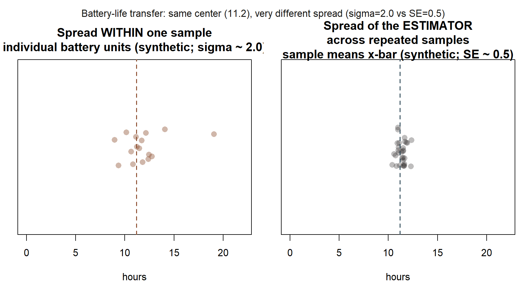
Suppose a reviewer wants to estimate the true average battery life of a new device model. The reviewer tests a small sample of \(n = 16\) units and records how many hours each lasts under a standard usage test, obtaining a sample mean of \(\bar{x} = 11.2\) hours. Based on the manufacturer’s historical testing across many similar device generations, the population standard deviation of individual battery life is treated as known, \(\sigma = 2.0\) hours (a known-SD simplification, exactly the same teaching device used for the MAC visit- duration example above).

The estimator here is \(\hat{\mu} = \bar{x}\), and its standard error is \[SE(\bar{x}) = \frac{\sigma}{\sqrt{n}} = \frac{2.0}{\sqrt{16}} = \frac{2.0}{4} = 0.5 \text{ hours}.\]

So the reviewer’s estimate of average battery life is 11.2 hours, with a standard error of 0.5 hours: if the reviewer tested a fresh batch of 16 units over and over, the resulting sample-mean battery-life estimates would typically sit about half an hour from the true average. Note what this is not: it is not a claim that any single unit’s battery lasts within half an hour of 11.2 hours — individual units vary by roughly 2 hours (that is \(\sigma\), the data-level spread); it is the average of 16 units that varies far less, because averaging cancels out much of the individual-unit noise. This is exactly the same \(\sigma/\sqrt{n}\) logic as the MAC visit-duration example, transplanted into a new context to check that you can apply the formula outside its original setting.

Figure 5: The same SE-vs-sample-SD contrast, transferred to the battery-life example (synthetic). Left: individual battery units scattered around \(\bar{x}=11.2\) hours with spread \(\sigma \approx 2.0\). Right: sample means from repeated 16-unit samples scattered around the same center with spread \(SE \approx 0.5\).

A common mistake

Reporting the sample SD when a standard error is called for, or vice versa. It is extremely common to see a sentence like “the average visit duration was 49.8 minutes (SD = 2.5),” which silently swaps in the standard error where the sample SD belongs, understating how variable individual visits actually are (the real sample SD is \(s = 15.2\) minutes — see Week 10, where this exact value returns for the bootstrap). The reverse mistake also happens: reporting \(\sigma = 15\) or \(s = 15.2\) as if it described the precision of the mean estimate, which wildly overstates the uncertainty in \(\bar{x}\) (the mean’s actual uncertainty is the much smaller \(SE(\bar{x}) = 2.5\)). The fix is always the same question: am I describing one observation, or a summary statistic computed from many observations? Individual-observation spread is \(\sigma\) or \(s\); summary- statistic spread is a standard error. The two will almost never be equal, and conflating them misleads a reader about precisely the thing a standard error exists to communicate honestly.

Low-stakes self-checks (ungraded)

• In your own words, explain the difference between an estimator and an estimate. Give one example of each using the MAC visit-duration sample.
• The MAC visit-duration sample has \(n = 36\), \(\bar{x} = 49.8\), and (known-\(\sigma\) simplification) \(\sigma = 15\). Recompute \(SE(\bar{x})\) by hand and confirm you get 2.5.
• Suppose the MAC Study had instead surveyed \(n = 400\) students (four times as many) and still observed \(\hat{p} = 0.38\). Recompute \(SE(\hat{p})\) for this larger sample size, and compare it to the \(n = 100\) value of about 0.0485. Is it a quarter as large? Why or why not?
• In the battery-life transfer example, if the reviewer had tested \(n = 64\) units instead of 16 (keeping \(\bar{x} = 11.2\) and \(\sigma = 2.0\) the same), what would \(SE(\bar{x})\) become?
• Write one sentence describing what \(SE(\hat{p}) \approx 0.0485\) means, and one separate sentence describing what it does not mean, for the MAC usage-rate survey.

Reading and source pointer

This week’s development follows MIT OCW 18.05’s treatment of estimators and standard error, used selectively as this course’s primary spine. As an optional, lighter pass over the same estimator/standard-error ideas, you may also look at OpenIntro IMS’s introductory inference material — useful if you want a gentler second explanation, but not required reading. These notes are the course’s own synthesis, grounded in but not copied from the sources.

Public vs. graded

These notes, the examples, and the practice here are public and ungraded — study material only. No graded prompts, answer keys, rubrics, point values, or due dates appear on this site. Graded inference checkpoints, quizzes, homework, labs, the midterm, the project, and the final live in Blackboard (the LMS), which is authoritative for due dates, submissions, and grades. If this page and Blackboard ever disagree, follow Blackboard.

Looking ahead

Week 4 puts the estimator concept to further work, asking a new question about it: is an estimator centered where it should be (bias), and how do bias and variance combine into a single measure of overall estimator quality (mean squared error)? The same MAC visit-duration sample reappears there in a bias/variance/MSE demonstration. Standard errors computed this week resurface directly in Week 7’s confidence intervals and Week 8’s hypothesis tests, so the SE(x̄) = 2.5 and SE(p̂) ≈ 0.0485 values above are worth keeping close at hand.

See also

• Week 2 — Sampling distributions and simulation
• Week 4 — Bias, variance, and mean squared error
• Week 7 — Confidence intervals (and midterm)
• Notation glossary
• Inference formula reference