set.seed(35103)
# Synthetic call-center hourly arrival counts (transfer example, not the MAC Study)
calls_per_hour <- c(4, 6, 5, 7, 3, 5)
lambda_hat <- mean(calls_per_hour)
lambda_hat # matches the by-hand MLE: 5Week 6 — Maximum likelihood estimation
Turning the likelihood function into a single best estimate, by calculus
Mathematical goal
Week 5 built the likelihood function \(L(\theta)\) and compared its height at a few candidate values of \(\theta\) by hand. That is progress, but it is not yet an estimation procedure: nobody wants to guess three candidate values and see which is tallest. This week’s mathematical goal is to find the value of \(\theta\) that maximizes \(L(\theta)\) exactly, using calculus, so that “most likely value of \(\theta\)” becomes a formula you can compute directly from data rather than a comparison of guesses. The tool is the same in every case: take the log-likelihood, differentiate with respect to \(\theta\), set the derivative to zero, and solve. We carry that single tool through two distributions used all term (Binomial/Bernoulli and Normal with known \(\sigma\)) and one transfer distribution (Poisson), and show that it always produces the intuitive estimator you would have guessed anyway — which is exactly the point of doing the derivation once, carefully.
The week question
If \(L(\theta)\) measures how well each candidate value of \(\theta\) explains the data you actually observed, what is the value of \(\theta\) that explains the data best, and how do you find it without checking candidates one at a time?
Notation
| Symbol | Meaning |
|---|---|
| \(\theta\) | Generic unknown parameter being estimated |
| \(L(\theta)\) | Likelihood function: joint density/pmf of the observed data, viewed as a function of \(\theta\) for fixed data |
| \(\ell(\theta) = \ln L(\theta)\) | Log-likelihood function |
| \(\hat\theta_{MLE}\) | Maximum likelihood estimate: the value of \(\theta\) that maximizes \(L(\theta)\) (equivalently \(\ell(\theta)\)) |
| \(\pi\), \(\hat\pi\) | Population proportion; its MLE |
| \(n\), \(k\) | Sample size; count of “successes” in a Binomial/Bernoulli sample |
| \(\mu\), \(\hat\mu\) | Population mean (Normal, \(\sigma\) known); its MLE |
| \(x_i\), \(\bar x\) | Individual observation; sample mean |
| \(\lambda\), \(\hat\lambda\) | Poisson rate parameter; its MLE |
| \(\dfrac{d\ell}{d\theta}\) | Derivative of the log-likelihood with respect to \(\theta\) — set to 0 to locate the maximum |
Conceptual setup
Two facts make maximizing a likelihood function tractable, and both are worth stating before any algebra.
Fact 1 — maximizing \(L(\theta)\) and maximizing \(\ell(\theta) = \ln L(\theta)\) give the same \(\hat\theta\). The natural log is a strictly increasing function, so it never changes which input produces the largest output: if \(L(\theta)\) peaks at some value, \(\ln L(\theta)\) peaks at that same value. This matters because raw likelihoods for independent data are products (one factor per observation), and products of many terms are awkward to differentiate. Logs turn those products into sums, and sums differentiate one term at a time. This is why every derivation below works with \(\ell(\theta)\), never \(L(\theta)\) directly.
Fact 2 — a maximum of a smooth function occurs where its derivative is zero (and the function is concave there). This is ordinary single-variable calculus, not anything special to statistics. The recipe is always the same three moves:
- Write down \(L(\theta)\) from the assumed model and the observed data.
- Take \(\ell(\theta) = \ln L(\theta)\), simplify.
- Differentiate \(\ell(\theta)\) with respect to \(\theta\), set \(\dfrac{d\ell}{d\theta} = 0\), and solve for \(\theta\). Call the solution \(\hat\theta_{MLE}\).
A full course in mathematical statistics would also check the second derivative is negative (confirming a maximum, not a minimum or saddle point) and check the boundary of the parameter space; for the two models this week, the log-likelihood is a smooth, single-peaked (concave) function of \(\theta\) over its whole valid range, so the first-order condition alone is what we need to see the idea. That verification is noted here and left as a background fact, not re-derived symbol by symbol on the page.
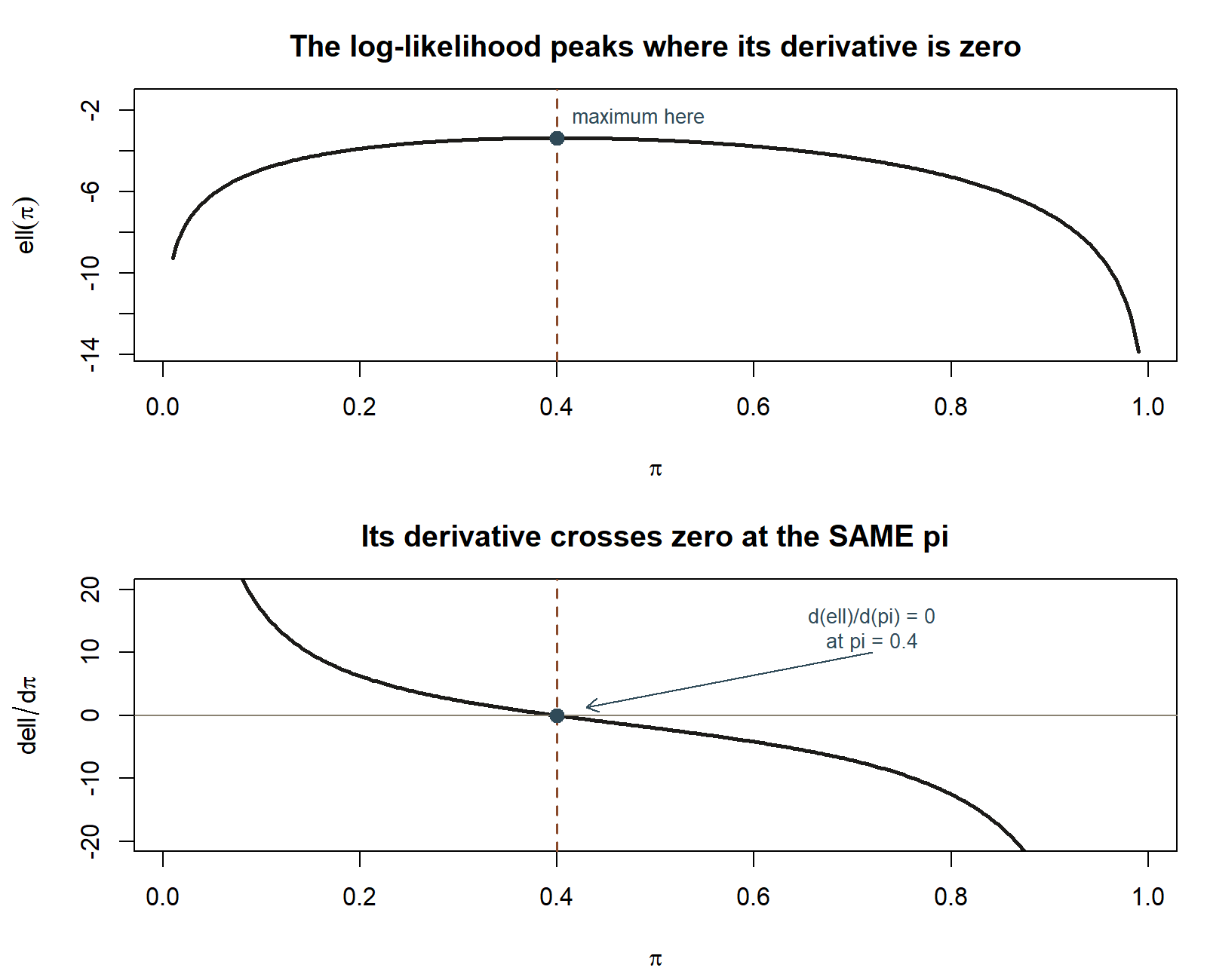
One more thing this week’s convention warning will return to: the likelihood is a function of \(\theta\), not a probability distribution over \(\theta\). Nothing about “maximizing \(L(\theta)\)” means \(\theta\) is random or that \(\hat\theta_{MLE}\) is “the most probable value of \(\theta\)” in a probability sense — that reading only becomes available once a prior is introduced in Week 12’s Bayesian framework.
Worked example
Worked example 1 — Binomial/Bernoulli MLE (the recurring MAC-Study pilot)
Symbolic derivation. Suppose \(n\) independent Bernoulli\((\pi)\) trials produce \(k\) successes. As in Week 5, the likelihood kernel (the part of \(L(\pi)\) that depends on \(\pi\)) is
\[ L(\pi) \propto \pi^{k}(1-\pi)^{n-k}, \qquad 0 < \pi < 1. \]
Take the log:
\[ \ell(\pi) = \ln L(\pi) = k\ln \pi + (n-k)\ln(1-\pi) + C, \]
where \(C\) collects constants that do not involve \(\pi\) (they vanish under differentiation). Differentiate with respect to \(\pi\):
\[ \frac{d\ell}{d\pi} = \frac{k}{\pi} - \frac{n-k}{1-\pi}. \]
Set this equal to zero and solve:
\[ \frac{k}{\pi} = \frac{n-k}{1-\pi} \;\;\Longrightarrow\;\; k(1-\pi) = (n-k)\pi \;\;\Longrightarrow\;\; k - k\pi = n\pi - k\pi \;\;\Longrightarrow\;\; k = n\pi. \]
\[ \boxed{\hat\pi_{MLE} = \frac{k}{n}} \]
That is exactly the sample proportion — the number every intro-stats student already computes, now justified as the value that makes the observed data most likely under the Bernoulli/Binomial model.
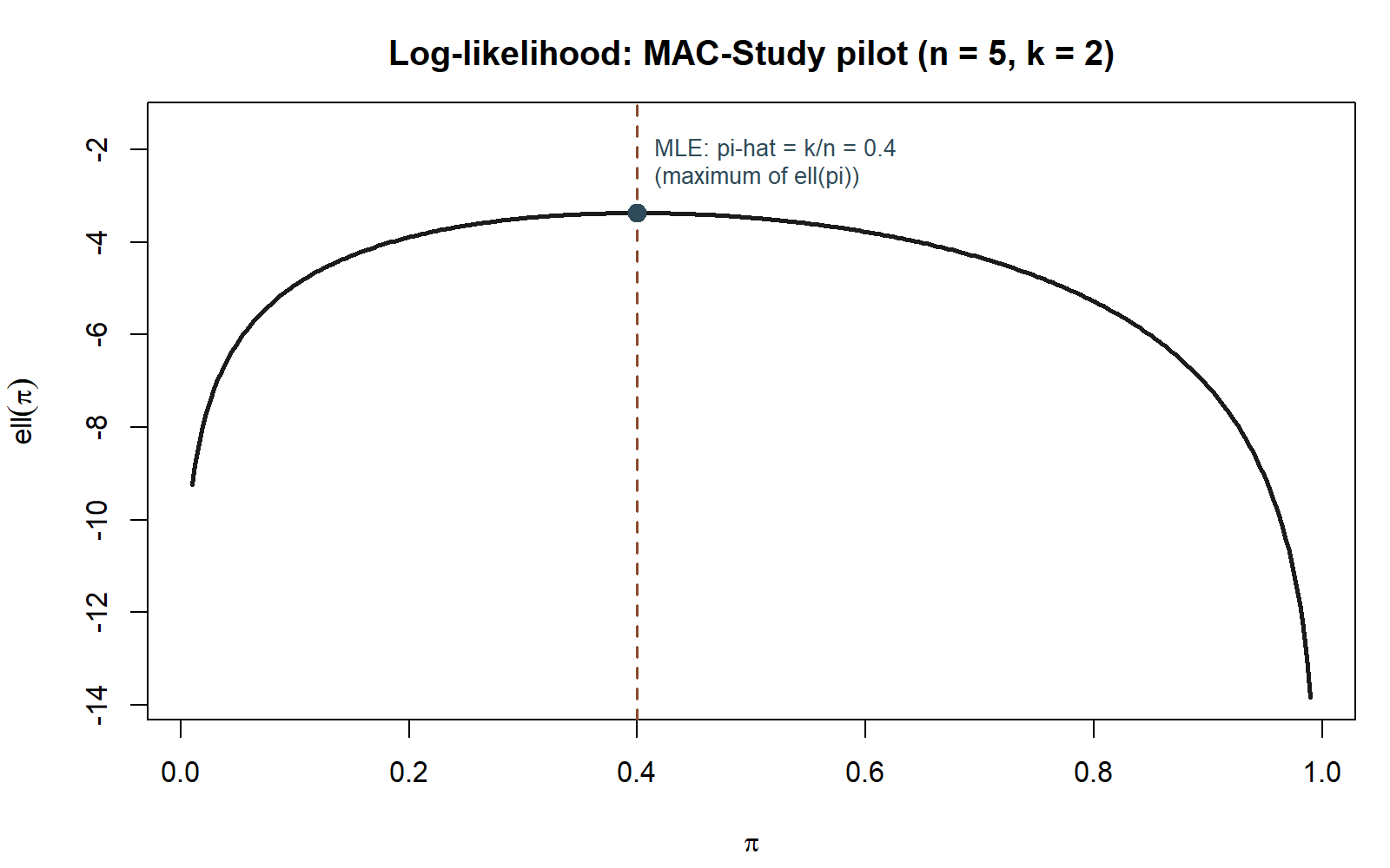
Numeric application (the pilot batch). Using the course’s locked small illustrative pilot — the first five survey responses, \(n = 5\), \(k = 2\) used the MAC:
\[ \hat\pi_{MLE} = \frac{k}{n} = \frac{2}{5} = 0.4. \]
This matches Week 5’s likelihood-kernel comparison exactly: among \(\pi = 0.2, 0.4, 0.6\), the kernel \(\pi^2(1-\pi)^3\) was tallest at \(\pi = 0.4\) (kernel values \(0.02048\), \(0.03456\), \(0.02304\) respectively). The calculus confirms that \(0.4\) is not just the tallest of those three candidates — it is the single tallest point over the entire interval \((0,1)\).
Worked example 2 — Normal MLE, \(\sigma\) known (the recurring MAC-Study pilot)
Symbolic derivation. Suppose \(x_1, \dots, x_n\) are independent draws from a Normal\((\mu, \sigma^2)\) distribution with \(\sigma\) treated as known (the course’s standing “known-\(\sigma\)” teaching simplification, same as Weeks 2–9). The likelihood is the product of the \(n\) Normal densities:
\[ L(\mu) = \prod_{i=1}^{n} \frac{1}{\sqrt{2\pi\sigma^2}} \exp\!\left(-\frac{(x_i-\mu)^2}{2\sigma^2}\right). \]
Take the log, turning the product into a sum:
\[ \ell(\mu) = -\frac{n}{2}\ln(2\pi\sigma^2) - \frac{1}{2\sigma^2}\sum_{i=1}^{n} (x_i - \mu)^2. \]
The first term does not involve \(\mu\), so only the second term matters for differentiation. Differentiate with respect to \(\mu\):
\[ \frac{d\ell}{d\mu} = \frac{1}{\sigma^2}\sum_{i=1}^{n} (x_i - \mu). \]
Set this equal to zero (note \(\sigma^2 > 0\), so it can be cleared without changing the solution):
\[ \sum_{i=1}^{n} (x_i - \mu) = 0 \;\;\Longrightarrow\;\; \sum_{i=1}^{n} x_i = n\mu. \]
\[ \boxed{\hat\mu_{MLE} = \frac{1}{n}\sum_{i=1}^{n} x_i = \bar x} \]
Once again, the calculus recovers the estimator every student already uses by instinct — the sample mean — now derived rather than assumed.
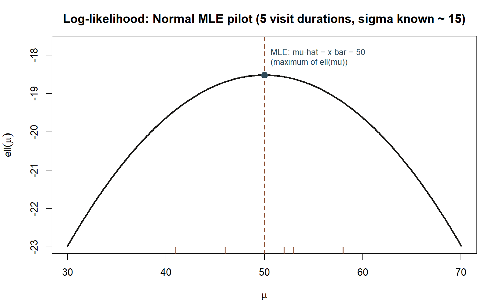
Numeric application (the pilot batch). The course’s locked small illustrative sample of five visit durations (minutes), a different pilot batch from the \(n = 36\) visit-duration sample used from Week 2 onward: \(52, 46, 58, 41, 53\).
\[ \hat\mu_{MLE} = \bar x = \frac{52 + 46 + 58 + 41 + 53}{5} = \frac{250}{5} = 50 \text{ minutes.} \]
Transfer example — Poisson MLE for a call-center arrival rate (synthetic; seed set)
Setting. A call center tracks the number of customer calls arriving per hour. A standard model for “count of events per fixed unit of time” is the Poisson distribution with rate parameter \(\lambda\): for a single hour, \(P(X = x) = \dfrac{e^{-\lambda}\lambda^{x}}{x!}\), \(x = 0, 1, 2, \dots\). This is a genuinely different sampling model from both examples above (support on all non-negative integers, one parameter that is simultaneously the mean and the variance), which is exactly why it is useful as a transfer case: the same three-step recipe applies unchanged.
Symbolic derivation. For \(n\) independent hours with observed counts \(x_1, \dots, x_n\), the likelihood is
\[ L(\lambda) = \prod_{i=1}^{n} \frac{e^{-\lambda}\lambda^{x_i}}{x_i!} = \frac{e^{-n\lambda}\,\lambda^{\sum x_i}}{\prod_{i=1}^n x_i!}. \]
Take the log:
\[ \ell(\lambda) = -n\lambda + \left(\sum_{i=1}^{n} x_i\right)\ln \lambda - \ln\!\left(\prod_{i=1}^n x_i!\right), \]
where the last term does not involve \(\lambda\). Differentiate with respect to \(\lambda\):
\[ \frac{d\ell}{d\lambda} = -n + \frac{\sum_{i=1}^{n} x_i}{\lambda}. \]
Set this equal to zero and solve:
\[ \frac{\sum_{i=1}^{n} x_i}{\lambda} = n \;\;\Longrightarrow\;\; \sum_{i=1}^{n} x_i = n\lambda. \]
\[ \boxed{\hat\lambda_{MLE} = \frac{1}{n}\sum_{i=1}^{n} x_i = \bar x} \]
The Poisson MLE for the rate is the sample mean count per hour — the same “average the data” shape as the Normal-mean derivation above, arrived at by the identical three-step recipe applied to a different model.
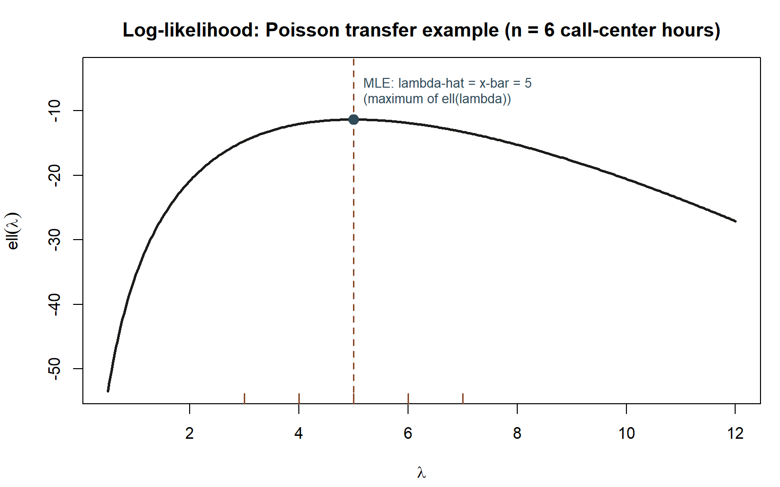
Numeric application (synthetic; seed 35103 set). Suppose the call center records the following number of calls in each of \(n = 6\) observed hours: \(4, 6, 5, 7, 3, 5\).
\[ \hat\lambda_{MLE} = \bar x = \frac{4+6+5+7+3+5}{6} = \frac{30}{6} = 5 \text{ calls per hour.} \]
This chunk is shown but not executed on this page (eval: false) — it only confirms the single number lambda_hat. The figure below goes one step further: it plots the full log-likelihood \(\ell(\lambda)\) this chunk’s data implies, over a grid of candidate \(\lambda\) values, so the boxed MLE above is visible as a maximum rather than just a printed number.
A convention warning
\(L(\theta)\) and \(\ell(\theta)\) are functions of the unknown parameter \(\theta\) for data that are already fixed — they are not probability distributions over \(\theta\), and \(\theta\) is not being treated as random when you maximize them. “The value of \(\theta\) that maximizes the likelihood” is a well-defined calculus question with a single answer; it is not the same claim as “the probability that \(\theta\) equals this value,” which requires a prior distribution on \(\theta\) and does not appear until Bayesian inference in Week 12. Keep maximum likelihood estimation and Bayesian posterior reasoning visually and verbally distinct: an MLE is a number derived from calculus on fixed data; a posterior is an entire distribution that requires a prior to exist in the first place.
A second, easily-missed warning: maximizing \(\ell(\theta)\) instead of \(L(\theta)\) is a convenience, not a different target. Because \(\ln(\cdot)\) is strictly increasing, the two maximizations always agree on \(\hat\theta_{MLE}\) — but they do not agree on the maximized height (the log-likelihood’s maximum value is \(\ln\) of the likelihood’s maximum value, not the same number). Only the location of the peak transfers; the peak’s height does not.
Practice (ungraded)
Self-check only — no submission, no key, no due date.
- Re-derive \(\hat\pi_{MLE} = k/n\) starting from \(\ell(\pi) = k\ln\pi + (n-k)\ln(1-\pi)\), writing out every algebra step from the derivative to the boxed result, without looking at the derivation above.
- A different pilot batch of Bernoulli MAC-usage responses has \(n = 8\) trials with \(k = 3\) successes. Using the boxed formula \(\hat\pi_{MLE} = k/n\), compute \(\hat\pi_{MLE}\) for this batch. (This is a self-check number only, not a new locked course fact.)
- For the Normal-mean derivation, explain in one or two sentences why the term \(-\frac{n}{2}\ln(2\pi\sigma^2)\) can be dropped before differentiating with respect to \(\mu\), but would not be droppable if you were instead solving for \(\hat\sigma_{MLE}\) with \(\mu\) known.
- Using the transfer example’s recipe, suppose a second call-center sample of \(n = 4\) hours gives counts \(2, 2, 3, 5\). Compute \(\hat\lambda_{MLE}\) by hand and state what it means in words (calls per hour).
- Explain, in your own words, why maximizing \(\ell(\theta) = \ln L(\theta)\) instead of \(L(\theta)\) directly changes none of the three boxed MLE results above.
Reading and source pointer
This week follows MIT OCW 18.05’s treatment of maximum likelihood estimation, which supports deriving the MLE by differentiating the log-likelihood and setting it to zero for both discrete (Binomial/Bernoulli) and continuous (Normal) models — the same differentiate-and-solve recipe used for the Poisson transfer example above. These notes are the course’s own synthesis, grounded in but not copied from the sources.
Public vs. graded
These notes, the examples, and the practice here are public and ungraded — study material only. No graded prompts, answer keys, rubrics, point values, or due dates appear on this site. Graded inference checkpoints, quizzes, homework, labs, the midterm, the project, and the final live in Blackboard (the LMS), which is authoritative for due dates, submissions, and grades. If this page and Blackboard ever disagree, follow Blackboard.
Looking ahead
Week 7 puts point estimates like \(\hat\pi_{MLE}\) and \(\hat\mu_{MLE}\) inside an interval that communicates uncertainty — the confidence interval — and also marks the in-class midterm (first-half material: sampling distributions through confidence intervals). The MLE machinery built this week does not stop at Week 7, either: point estimation by maximizing a likelihood is the same idea threading through hypothesis testing (Week 8), power (Week 9), and the Bayesian posterior mode (Week 12), where a prior is finally added to the picture this week deliberately withheld.
See also
- Week 5 — Likelihood
- Week 7 — Confidence intervals (+ midterm)
- Lab 06 — Likelihood curves — plots the sharper likelihood curve from the larger \(n = 100\), \(k = 38\) survey, peaked at \(\hat\pi = 0.38\), alongside this week’s calculus.
- Notation glossary
- Inference formula reference