Lab 10 — Bootstrap intervals

Building a percentile confidence interval by resampling, by hand, in base R

Purpose. This lab is the hands-on companion to Week 10 — Bootstrap inference. The week note develops the percentile bootstrap conceptually and compares it to the Week 7 theoretical confidence interval; this lab carries that same idea out step by step in code, so you can watch a bootstrap distribution build itself one resample at a time.

The idea

A confidence interval built from a formula, like the Week 7 interval for the MAC Study’s mean visit duration, leans on a theoretical result: if you know (or are willing to assume) the shape of the sampling distribution of \(\bar{x}\), you can write down its standard error directly and use a normal quantile to build the interval. The bootstrap takes a different route. It says: you do not actually have the population, and you do not want to lean on a normal-theory formula for the standard error of some more complicated statistic — so instead, treat the sample itself as a stand-in for the population, and repeatedly resample from it, with replacement, to see how much a statistic computed from a sample of this size actually bounces around.

Concretely: draw a new sample of size \(n\) from your original \(n\) observations, sampling with replacement (so the same original observation can appear zero, one, or several times in a given resample). Compute the statistic of interest — here, the mean — on that resample. Repeat this thousands of times. The resulting collection of resample means is the bootstrap distribution of \(\bar{x}\). Its spread approximates the true sampling distribution’s spread, and its middle 95% (the 2.5th to 97.5th percentile) gives a percentile bootstrap confidence interval — no normal-theory formula required.

This lab uses base R only, following this course’s house convention (sample(), replicate(), and friends) rather than the infer-package pipeline that ModernDive’s own examples use. The framing — build the sampling distribution of a statistic by simulation rather than by formula — is exactly ModernDive’s simulation-based approach; we are just writing it out in base R instead of specify() |> generate() |> calculate().

Goal

By the end of this lab you will have:

1. Constructed a synthetic stand-in sample for the MAC Study’s \(n = 36\) visit-duration sample.
2. Drawn \(B = 2000\) bootstrap resamples from it, with replacement, and computed the mean of each.
3. Read off the 2.5th and 97.5th percentiles of the bootstrap distribution of means as a 95% percentile confidence interval.
4. Compared that bootstrap interval to the Week 7 theoretical confidence interval, \((44.9, 54.7)\).

Setup

All chunks below are shown with #| eval: false — this build presents code as teaching material, not as executed output. When you run this in your own R or Posit Cloud session, keep set.seed(35103) at the top so your results are reproducible and comparable to a classmate’s.

set.seed(35103)

# No external packages needed — base R only, per course convention.

A note on the data before you start: the MAC Study’s real recorded sample is \(n = 36\) visits with sample mean \(\bar{x} = 49.8\) minutes and sample SD \(s = 15.2\) minutes (Week 7, Week 10). This lab does not have access to the 36 individual recorded visit lengths — only their summary. So Step 1 below builds a synthetic stand-in vector: 36 numbers, drawn from a normal model, engineered to have (very nearly) the same mean and SD as the real sample. This stand-in is clearly a teaching device, not the real data — but it behaves the same way under resampling, which is all this lab needs.

Steps

Step 1 — Build a synthetic stand-in sample

Generate 36 synthetic values from a Normal(49.8, 15.2) model. This is not the real recorded sample of 36 MAC visits — it is a synthetic vector engineered to share the real sample’s mean and SD, standing in for it so the resampling mechanics below have something concrete to work on.

set.seed(35103)

# Synthetic stand-in for the real n = 36 visit-duration sample.
# Engineered to share the real sample's summary: mean 49.8, SD 15.2.
visit_sample <- rnorm(36, mean = 49.8, sd = 15.2)

length(visit_sample)   # should be 36
mean(visit_sample)     # near 49.8, not exactly (rnorm() draws are random)
sd(visit_sample)       # near 15.2, not exactly

This chunk is shown but not executed on this page (eval: false) — running it yourself is the point. The figure below was produced by running exactly this chunk’s code separately (same seed 35103, same rnorm(36, mean = 49.8, sd = 15.2) call), so you can see what visit_sample actually looks like as 36 points rather than only as two summary numbers:

Figure 1: The synthetic stand-in sample, visualized (synthetic). 36 points drawn from Normal(49.8, 15.2), the stand-in this lab treats as “the sample in hand.” The dashed line marks this particular draw’s mean (49.09), close to but not exactly the 49.8 target.

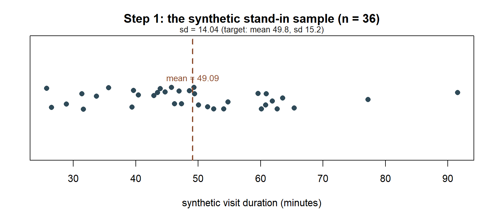
Because rnorm() draws are random, mean(visit_sample) and sd(visit_sample) will land close to 49.8 and 15.2 but not hit them exactly — that is expected and fine. What matters for the rest of this lab is that visit_sample is a length-36 numeric vector in the right neighborhood, which we now treat as “the sample in hand” for resampling purposes.

Step 2 — Draw one bootstrap resample

Before automating thousands of resamples, look at a single one. Sample 36 values from visit_sample, with replacement, and compute the mean of that resample.

set.seed(35103)

one_resample <- sample(visit_sample, size = 36, replace = TRUE)

length(one_resample)     # still 36 — same size as the original
mean(one_resample)       # a single bootstrap replicate of the mean

This chunk is shown but not executed on this page — running it yourself is the point. The figure below was produced by running exactly this chunk’s code separately (same seed 35103), then counting how many times each of the 36 original values landed in one_resample, so you can see “with replacement” as a picture rather than only as a phrase:

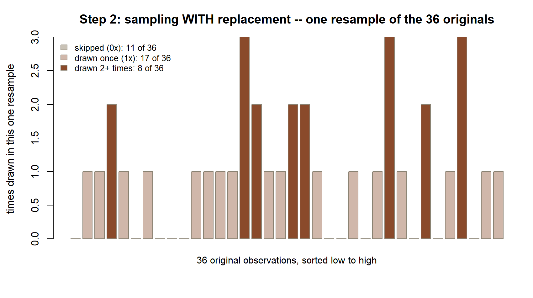
Figure 2: Sampling with replacement, made visible (synthetic). For this one resample, 11 of the 36 originals were skipped entirely (drawn 0 times), 17 were drawn exactly once, and 8 were drawn two or more times — exactly the mechanism replace = TRUE produces.

Notice replace = TRUE is doing the essential work here: without it, sample() would just reshuffle the same 36 values in a different order and every resample mean would come out identical to mean(visit_sample). With replacement, some original values are skipped in a given resample and others are drawn two, three, or more times, so the resample mean genuinely varies from resample to resample. That variation is exactly what the bootstrap is measuring.

Step 3 — Automate B = 2000 bootstrap resamples

Use replicate() to repeat Step 2’s logic 2000 times, storing each resample’s mean.

set.seed(35103)

B <- 2000

boot_means <- replicate(
  B,
  mean(sample(visit_sample, size = 36, replace = TRUE))
)

length(boot_means)   # should be 2000
head(boot_means)      # first few bootstrap replicate means
mean(boot_means)      # center of the bootstrap distribution
sd(boot_means)        # bootstrap standard error of the mean

boot_means is now a vector of 2000 numbers, each one the mean of an independent resample-with-replacement of size 36 drawn from visit_sample. This vector is the bootstrap distribution. Its standard deviation, sd(boot_means), is the bootstrap standard error — an estimate of how much \(\bar{x}\) would vary from sample to sample, built entirely by resampling rather than by a formula. It should land in the neighborhood of \(s/\sqrt{n} = 15.2/6 \approx 2.53\), the bootstrap SE reported in the Week 10 note, though the exact value will depend on the particular visit_sample draw from Step 1.

This chunk is shown but not executed on this page. The figure below extends this chunk’s already-computed boot_means with a plotting call not written on the page — tracking the cumulative mean and SD as resamples accumulate, produced by running exactly this chunk’s code separately (same seed, same B = 2000), so you can watch both settle down toward a stable value rather than only reading off their final numbers:

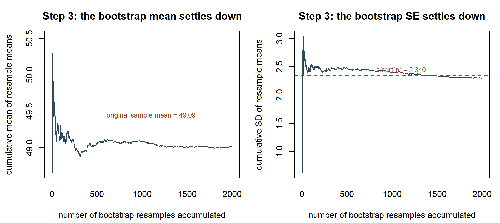
Figure 3: Bootstrap replication converging (synthetic). As the number of accumulated resamples grows from 1 to 2000, the running mean of boot_means settles near the original sample mean (left), and the running SD settles near the theoretical standard error \(s/\sqrt{n} \approx 2.34\) (right) — this settling-down is what “repeat this thousands of times” is buying.

See the distribution, not just its summary. A histogram of boot_means is the actual pedagogical payoff of this lab: watching 2000 resample means pile up into a distribution, rather than only reading off two summary numbers.

hist(boot_means, breaks = 40,
     main = "Bootstrap distribution of the mean (B = 2000 resamples)",
     xlab = "resample mean visit duration (minutes)")
abline(v = mean(visit_sample), lty = 2)   # centered near the original sample mean, ~49.8

What this shows (public-safe description, since this chunk is not executed here): a roughly bell-shaped histogram of the 2000 resample means, centered near the original sample mean (\(\approx 49.8\), marked by the dashed line) and spread out by roughly sd(boot_means) in either direction — this shape is the bootstrap distribution Step 4 reads its percentile interval from, made visible rather than only summarized by two numbers. The figure below was produced by running exactly this chunk’s hist()/abline() code separately (same seed, same boot_means), so you can check your prediction of its shape against a real result:

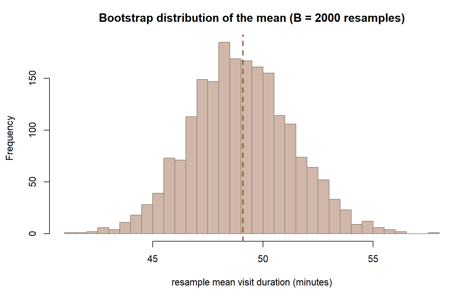
Figure 4: The bootstrap distribution, rendered (synthetic). A histogram of the 2000 bootstrap resample means, with a dashed line at the original sample mean (49.09 for this particular visit_sample draw). The bell shape and the spread are exactly what Step 4 reads its percentile interval from.

Step 4 — Read off the percentile confidence interval

The percentile bootstrap 95% confidence interval is simply the 2.5th and 97.5th percentiles of boot_means.

set.seed(35103)

boot_ci <- quantile(boot_means, probs = c(0.025, 0.975))

boot_ci

quantile(boot_means, probs = c(0.025, 0.975)) cuts off the lowest 2.5% and the highest 2.5% of the 2000 bootstrap means, leaving the middle 95% — read directly off the simulated distribution, with no normal-theory formula anywhere in sight. Compare the two numbers boot_ci prints to the Week 10 note’s reported percentile bootstrap interval, approximately \((44.84, 54.76)\), and to the Week 7 theoretical interval, \((44.9, 54.7)\). They should be close but not identical: the bootstrap interval is built from resampling a single synthetic stand-in sample, so its exact endpoints depend on that sample’s particular values and on which 2000 resamples happened to be drawn, while the Week 7 interval comes from a normal-theory formula using the known-\(\sigma\) simplification. Rerunning Steps 1–4 with a different seed would shift boot_ci slightly; the overall center and width should stay recognizably similar.

This chunk is shown but not executed on this page. The figure below extends this chunk’s boot_ci object with a comparison plot not written on the page, produced by running exactly this chunk’s code separately (same seed, same boot_means):

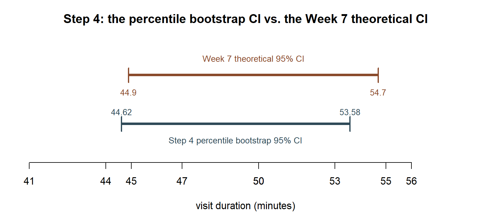
Figure 5: The percentile bootstrap CI vs. the Week 7 theoretical CI (synthetic). For this particular run, boot_ci = (44.62, 53.58) — close to, but not identical to, the Week 7 theoretical interval (44.9, 54.7); both are reported here rather than treating one as simply replacing the other.

Verify

Before treating your bootstrap interval as trustworthy, check all of the following in your own session:

• length(visit_sample) is exactly 36, and mean(visit_sample) / sd(visit_sample) land close to 49.8 and 15.2 respectively (not exact, but in the right neighborhood — large discrepancies mean Step 1 was not run correctly, or set.seed(35103) was skipped or placed inconsistently).
• length(boot_means) is exactly 2000 — one mean per bootstrap resample, no more, no fewer.
• boot_ci is a two-number interval with the lower bound below the upper bound, both numbers in the general neighborhood of the 40s-to-50s range (not, for instance, negative or in the hundreds — a sign something in Step 1 or Step 3 was mis-specified).
• The width of boot_ci (upper minus lower) is in the same rough neighborhood as the Week 7 interval’s width of \(54.7 - 44.9 = 9.8\) minutes — the bootstrap and theoretical intervals should agree approximately, not wildly diverge, because both are estimating the same quantity (the sampling variability of \(\bar{x}\) for \(n = 36\)) from consistent inputs.
• Re-running the whole script from set.seed(35103) at the top reproduces the same boot_ci numbers exactly — if it does not, some randomness-consuming step is happening before the seed is set, or out of order.

Consider a small, unrelated synthetic scenario, useful for sanity-checking the resampling logic without re-running code: a teaching lab (not the MAC Study) records 5 quiz-completion times, in minutes: \(8, 9, 11, 12, 15\) — synthetic numbers, not drawn from any real class. Their mean is \((8+9+11+12+15)/5 = 55/5 = 11\). One possible bootstrap resample of size 5, drawn with replacement, might be \(9, 11, 11, 8, 15\) (the value 11 happened to be drawn twice, and 12 was skipped this time); its mean is \((9+11+11+8+15)/5 = 54/5 = 10.8\). Another resample might draw \(8, 8, 12, 15, 15\), with mean \((8+8+12+15+15)/5 = 58/5 = 11.6\). Repeating this thousands of times and collecting the resample means builds a bootstrap distribution centered near 11, with spread reflecting how much a mean of 5 values drawn from this small pool can plausibly vary — exactly the same mechanism as Steps 2–4 above, just small enough to trace by hand for a couple of resamples. This synthetic 5-value example is unrelated to the MAC Study’s likelihood pilot batch from Weeks 5–6, which also happens to use 5 observations — the coincidence in size is not meaningful; the values and context here are freshly invented for this lab.

AI use note

Tool	Purpose	Verification
None used for this lab’s code or numbers	All base-R chunks, the synthetic stand-in sample, and the hand-traced transfer example were authored directly against this course’s own conventions	Every locked figure (the Week 7 interval \((44.9, 54.7)\), the Week 10 bootstrap interval \(\approx(44.84, 54.76)\), and the bootstrap SE \(\approx 2.53\)) was checked against the course’s own recurring-case numbers rather than re-derived; the transfer-example arithmetic was checked by hand (\(55/5=11\); \(54/5=10.8\); \(58/5=11.6\))

If you use an AI tool to help you debug or extend this lab in your own work, record what you asked it, what it returned, and how you checked the result before trusting it — the same two-column habit modeled above.

See also

• Week 10 — Bootstrap inference — the concept companion to this lab.
• Inference formula reference
• R & Quarto setup

The graded deliverable, its rubric, and due date live in Blackboard (the LMS) — this page is study and practice only.