Week 12 — Bayesian inference
Updating a belief about a parameter with data, and what a credible interval really claims
Mathematical goal
Derive the general rule for Bayesian updating — prior \(\pi(\theta)\) times likelihood \(L(\theta \mid \text{data})\) is proportional to posterior \(\pi(\theta \mid \text{data})\) — and then specialize that rule to the case this course has been building toward all term: a Beta prior on a proportion \(\pi\), updated by Binomial data. Prove that a \(\text{Beta}(a, b)\) prior combined with \(k\) successes in \(n\) Binomial trials produces a \(\text{Beta}(a + k,\, b + n - k)\) posterior — the Beta-Binomial conjugacy result — and use it to compute a posterior mean, posterior standard deviation, and an approximate credible interval for this course’s recurring usage-rate parameter.
The week question
Every framework this course has used so far treats the parameter \(\theta\) (whether written \(\mu\) or \(\pi\)) as a fixed, unknown constant, and asks what the data would look like under various possible values of \(\theta\) — that is exactly what the likelihood function \(L(\theta \mid \text{data})\) from Weeks 5 and 6 does. Bayesian inference asks a different question: instead of treating \(\theta\) as fixed and asking about the data, can we treat \(\theta\) itself as uncertain — describe our belief about it with a probability distribution — and then update that distribution once data arrive? This week derives exactly how that update works, shows it has a clean closed form for the Beta/Binomial pair this course has already been using, and works the update through on the MAC Study’s own usage-rate survey.
Notation
| Symbol | Meaning |
|---|---|
| \(\theta\) | the unknown parameter (here, a proportion, so also written \(\pi\) below) |
| \(\pi(\theta)\) | the prior density on \(\theta\) — belief about \(\theta\) before seeing this term’s data |
| \(L(\theta \mid \text{data})\) | the Bayesian likelihood — same function as Weeks 5–6’s \(L(\theta)\), now paired with a prior |
| \(\pi(\theta \mid \text{data})\) | the posterior density on \(\theta\) — updated belief after seeing the data |
| \(\text{Beta}(a, b)\) | the Beta distribution, with density \(\propto \theta^{a-1}(1-\theta)^{b-1}\) on \((0,1)\), mean \(a/(a+b)\) |
| \(n\) | number of Binomial trials (survey respondents) |
| \(k\) | number of successes observed (respondents who used the MAC) |
| \(\binom{n}{k}\) | the Binomial coefficient — a constant with respect to \(\theta\) |
| \(\propto\) | “proportional to” — equal up to a multiplicative constant that does not depend on \(\theta\) |
| \(\text{Var}(\theta \mid \text{data})\) | posterior variance of \(\theta\) |
| \(\Phi(\cdot)\) | standard normal cdf, used for the normal-approximation credible interval |
Conceptual setup
From likelihood alone to prior times likelihood. Weeks 5 and 6 built the Binomial likelihood for a proportion \(\pi\): if \(n\) independent trials produce \(k\) successes, the probability of that exact data pattern, viewed as a function of the unknown \(\pi\), is
\[ L(\pi \mid \text{data}) = \binom{n}{k}\pi^k(1-\pi)^{n-k}. \]
Weeks 5–6 used this function only to rank candidate values of \(\pi\) against each other (the likelihood-kernel comparison in Week 5, then the MLE \(\hat\pi = k/n\) in Week 6). At no point was \(L(\pi \mid \text{data})\) treated as a probability distribution over \(\pi\) — the notation ledger’s convention-risk flag is explicit about this: a likelihood is a function of \(\theta\) for fixed data, never a probability of \(\theta\).
Bayesian inference adds one new ingredient: a prior density \(\pi(\theta)\), representing a degree of belief about \(\theta\) before the current data are observed. (Context disambiguates the two uses of the symbol \(\pi\) here — \(\pi(\theta)\) is a density function of \(\theta\), while \(\pi\) alone, as in the rest of this section, is still this course’s usual symbol for the population proportion parameter. This double use is inherited directly from the standard notation and is flagged once, here, rather than repeated at every occurrence.) Once a prior exists, Bayes’ rule for densities gives the rule for turning a prior into a posterior:
\[ \pi(\theta \mid \text{data}) = \frac{L(\theta \mid \text{data})\,\pi(\theta)}{\int L(\theta \mid \text{data})\,\pi(\theta)\,d\theta}. \]
The denominator is a single number (once the data are fixed) — it does not depend on \(\theta\), since \(\theta\) has been integrated out. It exists purely to rescale the numerator so that \(\pi(\theta \mid \text{data})\) integrates to \(1\), as any proper density must. Because that denominator is a \(\theta\)-free constant, this relationship is almost always written using proportionality instead of full equality:
\[ \pi(\theta \mid \text{data}) \propto L(\theta \mid \text{data})\,\pi(\theta). \]
This is the central rule of Bayesian updating: posterior is proportional to likelihood times prior. In words — start with a belief about \(\theta\) (the prior), multiply it pointwise by how well each candidate value of \(\theta\) explains the observed data (the likelihood), and whatever shape results, once rescaled to integrate to \(1\), is the updated belief (the posterior). Everything that follows in this section is a matter of carrying out that multiplication for one specific, tractable pair of prior and likelihood.
Setting up the Beta-Binomial case. Suppose the prior on \(\pi\) is a \(\text{Beta}(a, b)\) distribution, whose density (up to the normalizing constant, which again does not involve \(\pi\)) is
\[ \pi(\pi) \propto \pi^{a-1}(1-\pi)^{b-1}, \qquad 0 < \pi < 1. \]
(As above, the left-hand \(\pi(\cdot)\) denotes the prior density and the argument \(\pi\) denotes the parameter — the same symbol carrying its usual double duty.) Suppose the data are \(n\) independent Binomial trials with \(k\) successes, so the likelihood is the Binomial form already derived in Weeks 5–6:
\[ L(\pi \mid \text{data}) = \binom{n}{k}\pi^k(1-\pi)^{n-k}. \]
Multiplying prior by likelihood. Apply the updating rule derived above:
\[ \pi(\pi \mid \text{data}) \propto L(\pi \mid \text{data})\,\pi(\pi) \propto \binom{n}{k}\pi^k(1-\pi)^{n-k} \cdot \pi^{a-1}(1-\pi)^{b-1}. \]
The factor \(\binom{n}{k}\) does not involve \(\pi\) at all, so it can be absorbed into the proportionality constant and dropped. Combine the remaining powers of \(\pi\) and of \((1-\pi)\) separately, since exponents of the same base add:
\[ \pi(\pi \mid \text{data}) \propto \pi^{k}\pi^{a-1}(1-\pi)^{n-k}(1-\pi)^{b-1} = \pi^{(a+k)-1}(1-\pi)^{(b+n-k)-1}. \]
Recognizing the result. This last expression is, up to a normalizing constant, exactly the density of a \(\text{Beta}(a+k,\, b+n-k)\) distribution — compare directly to the general Beta density \(\pi^{a'-1}(1-\pi)^{b'-1}\) with \(a' = a+k\) and \(b' = b+n-k\). Because a density is uniquely determined (up to its normalizing constant) by its functional form, and this functional form is exactly a Beta density, the posterior is that Beta distribution — no further integration is required to identify it:
\[ \pi \mid \text{data} \sim \text{Beta}(a+k,\ b+n-k). \]
This is the Beta-Binomial conjugacy result. “Conjugate” means the posterior belongs to the same family (Beta) as the prior — updating never leaves the Beta family, it only moves the two parameters. The update rule itself has a clean reading: start with \(a\) and \(b\), then add the observed successes to \(a\) and the observed failures to \(b\). A helpful interpretation of the prior parameters themselves falls out of this: \(a\) and \(b\) behave exactly like “prior successes” and “prior failures” — a \(\text{Beta}(a,b)\) prior carries the same updating weight as having already observed \(a\) successes and \(b\) failures in some earlier, hypothetical dataset of size \(a+b\). The larger \(a+b\) is, the more data it takes to move the posterior noticeably away from the prior mean.
Before working the MAC Study’s own numbers below, it helps to see the whole mechanism as one picture, using a small illustrative example distinct from the case this week’s worked example builds:
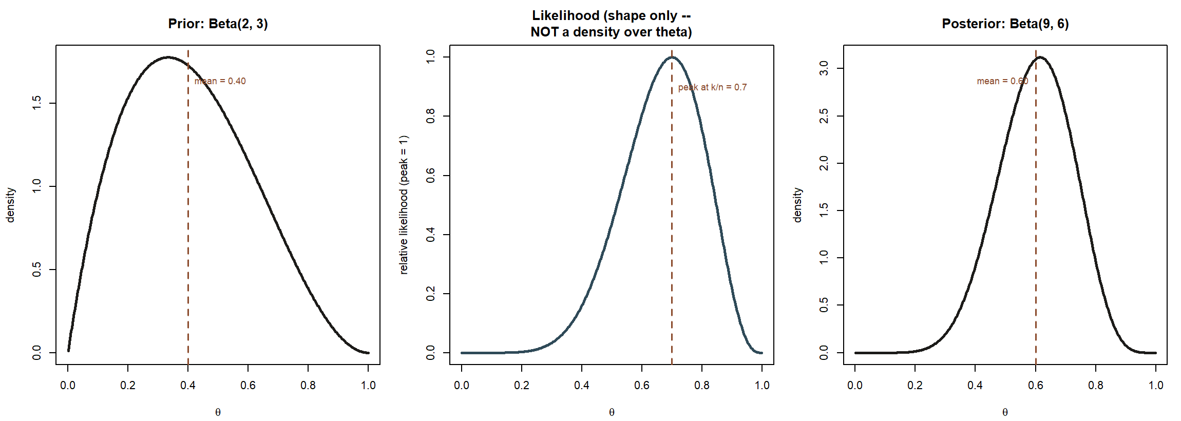
Posterior mean, as a weighted average. Since \(\text{Beta}(a', b')\) has mean \(a'/(a'+b')\), the posterior mean here is
\[ E[\pi \mid \text{data}] = \frac{a+k}{(a+k)+(b+n-k)} = \frac{a+k}{a+b+n}. \]
This can be rewritten to make the “weighted average” reading explicit. Let \(\pi_0 = a/(a+b)\) be the prior mean and \(\hat\pi = k/n\) be the sample proportion (the MLE from Week 6). A short algebraic rearrangement (not carried out in full here, since it is a standard identity) shows
\[ E[\pi \mid \text{data}] = \left(\frac{a+b}{a+b+n}\right)\pi_0 + \left(\frac{n}{a+b+n}\right)\hat\pi, \]
a weighted average of the prior mean and the sample proportion, with weights that shift toward the data as \(n\) grows relative to the prior’s “sample size” \(a+b\). As \(n \to \infty\) with \(a, b\) fixed, the posterior mean converges to \(\hat\pi\) — the data eventually dominate any fixed prior.
Worked example
MAC Study slice — updating the director’s belief about the usage rate.
Before this term’s survey, the MAC director’s belief about \(\pi\), the proportion of students who use the MAC in a given week, is represented by a \(\text{Beta}(a=3,\, b=7)\) prior. Its mean is
\[ E[\pi] = \frac{a}{a+b} = \frac{3}{10} = 0.30, \]
consistent with a director who expects roughly 30% weekly usage before seeing this term’s numbers, but whose prior is not extremely confident (a \(\text{Beta}(3,7)\) carries the updating weight of only \(a+b = 10\) hypothetical prior observations — a fairly weak prior, easily outweighed by real data).
The data are the full survey from Weeks 3–8: \(n = 100\) students, \(k = 38\) used the MAC. Applying the Beta-Binomial update derived above:
\[ \pi \mid \text{data} \sim \text{Beta}(a+k,\ b+n-k) = \text{Beta}(3+38,\ 7+100-38) = \text{Beta}(41, 69). \]
Posterior mean.
\[ E[\pi \mid \text{data}] = \frac{41}{41+69} = \frac{41}{110} \approx 0.373. \]
Checking this against the weighted-average form above: prior mean \(0.30\) gets weight \(10/110\), and sample proportion \(\hat\pi = 38/100 = 0.38\) gets weight \(100/110\) — so the posterior mean sits close to, but not exactly at, the sample proportion, pulled very slightly toward the prior. That is exactly the pattern the formula predicts: with \(n=100\) data points against only \(a+b=10\) prior “observations,” the data dominate almost entirely.
Posterior standard deviation. The variance of a \(\text{Beta}(a', b')\) distribution is \(\dfrac{a'b'}{(a'+b')^2(a'+b'+1)}\). With \(a'=41\), \(b'=69\), \(a'+b'=110\):
\[ \text{Var}(\pi \mid \text{data}) = \frac{(41)(69)}{(110)^2(111)} = \frac{2829}{110^2 \times 111}. \]
Computing the denominator: \(110^2 = 12{,}100\), and \(12{,}100 \times 111 = 1{,}343{,}100\). So
\[ \text{Var}(\pi \mid \text{data}) = \frac{2829}{1{,}343{,}100} \approx 0.002106, \]
\[ \text{SD}(\pi \mid \text{data}) = \sqrt{0.002106} \approx 0.0459. \]
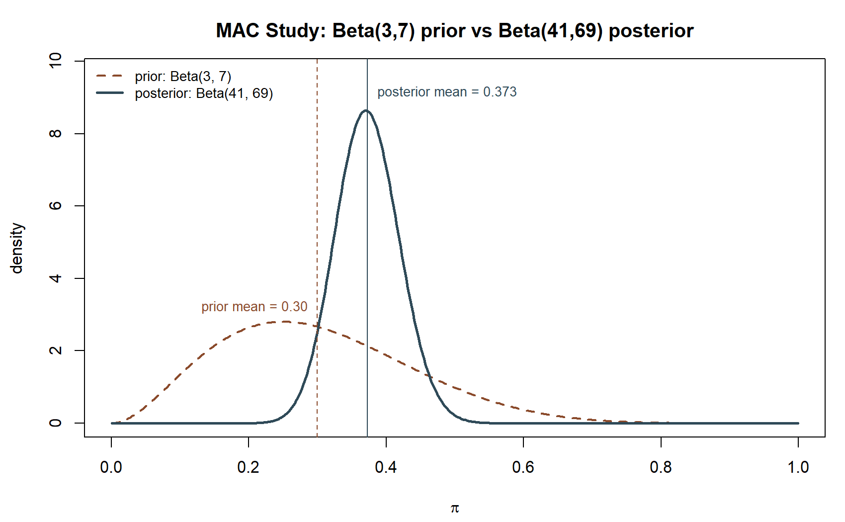
Seeing the update. Before turning the mean and SD into an interval, look at the prior and posterior as two curves on the same axis — this is the Beta-Binomial conjugacy result made visible for this week’s own numbers, rather than the illustrative pair above:
Normal-approximation 95% credible interval. For a Beta posterior this concentrated (both \(a'=41\) and \(b'=69\) are comfortably large), a normal approximation to the posterior is reasonable, exactly as the normal approximation was used for confidence intervals in Week 7:
\[ 0.373 \pm 1.96(0.0459) \approx 0.373 \pm 0.0900 \approx (0.283,\ 0.463). \]
A credible interval is a claim about area under the posterior curve, not just two endpoints computed from a formula — the picture below shades exactly that area:
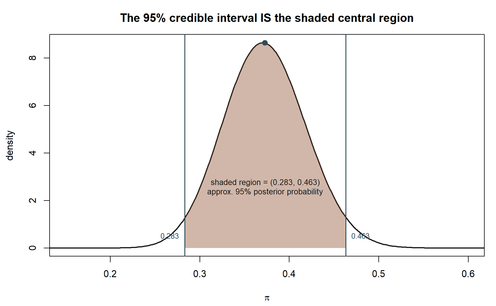
Table — the update at a glance. Reading prior and posterior side by side shows the update’s whole effect in one place — the numeric companion to the two figures above: the mean moves modestly (0.30 \(\to\) 0.373), the spread shrinks substantially, and the “effective sample size” \(a+b\) grows from 10 to 110 — a direct measure of how much more concentrated the belief becomes after 100 real observations are folded in.
| Quantity | Prior Beta(3, 7) | Posterior Beta(41, 69) |
|---|---|---|
| Mean | \(3/10 = 0.30\) | \(41/110 \approx 0.373\) |
| SD | \(\sqrt{\frac{(3)(7)}{10^2(11)}} \approx 0.138\) | \(\approx 0.0459\) |
| “Effective sample size” \(a+b\) | \(10\) | \(110\) |
| Interpretation | a director’s belief worth about 10 hypothetical prior observations | that belief plus 100 real survey responses, now much more concentrated |
The SD shrinking from about \(0.138\) to about \(0.046\) — roughly a threefold tightening — is the numeric signature of “the data dominated a comparatively weak prior,” the same story the mean’s modest shift from \(0.30\) to \(0.373\) already told in words above.
Transfer example (synthetic; seed set) — updating a coin’s bias with new flips.
Return to the coin-bias setting first introduced as a running device in Weeks 5–6 (the pilot survey’s likelihood-kernel comparison used the same Binomial machinery this week reuses). Suppose, as a fresh synthetic scenario distinct from the MAC Study, someone holds a weak prior belief that a particular coin is close to fair, represented as \(\text{Beta}(a=2,\, b=2)\) — mean \(2/4 = 0.50\), and, like the MAC director’s prior, carrying the weight of only \(a+b=4\) hypothetical prior flips.
New data arrive: \(n = 20\) new flips, \(k = 15\) heads. Applying the same conjugacy result:
\[ \theta \mid \text{data} \sim \text{Beta}(a+k,\ b+n-k) = \text{Beta}(2+15,\ 2+20-15) = \text{Beta}(17, 7). \]
Posterior mean:
\[ E[\theta \mid \text{data}] = \frac{17}{17+7} = \frac{17}{24} \approx 0.708. \]
Posterior variance and SD, using \(a'=17\), \(b'=7\), \(a'+b'=24\):
\[ \text{Var}(\theta \mid \text{data}) = \frac{(17)(7)}{(24)^2(25)} = \frac{119}{14{,}400} \approx 0.008264, \qquad \text{SD}(\theta \mid \text{data}) \approx 0.0909. \]
Normal-approximation 95% credible interval:
\[ 0.708 \pm 1.96(0.0909) \approx 0.708 \pm 0.178 \approx (0.530,\ 0.886). \]
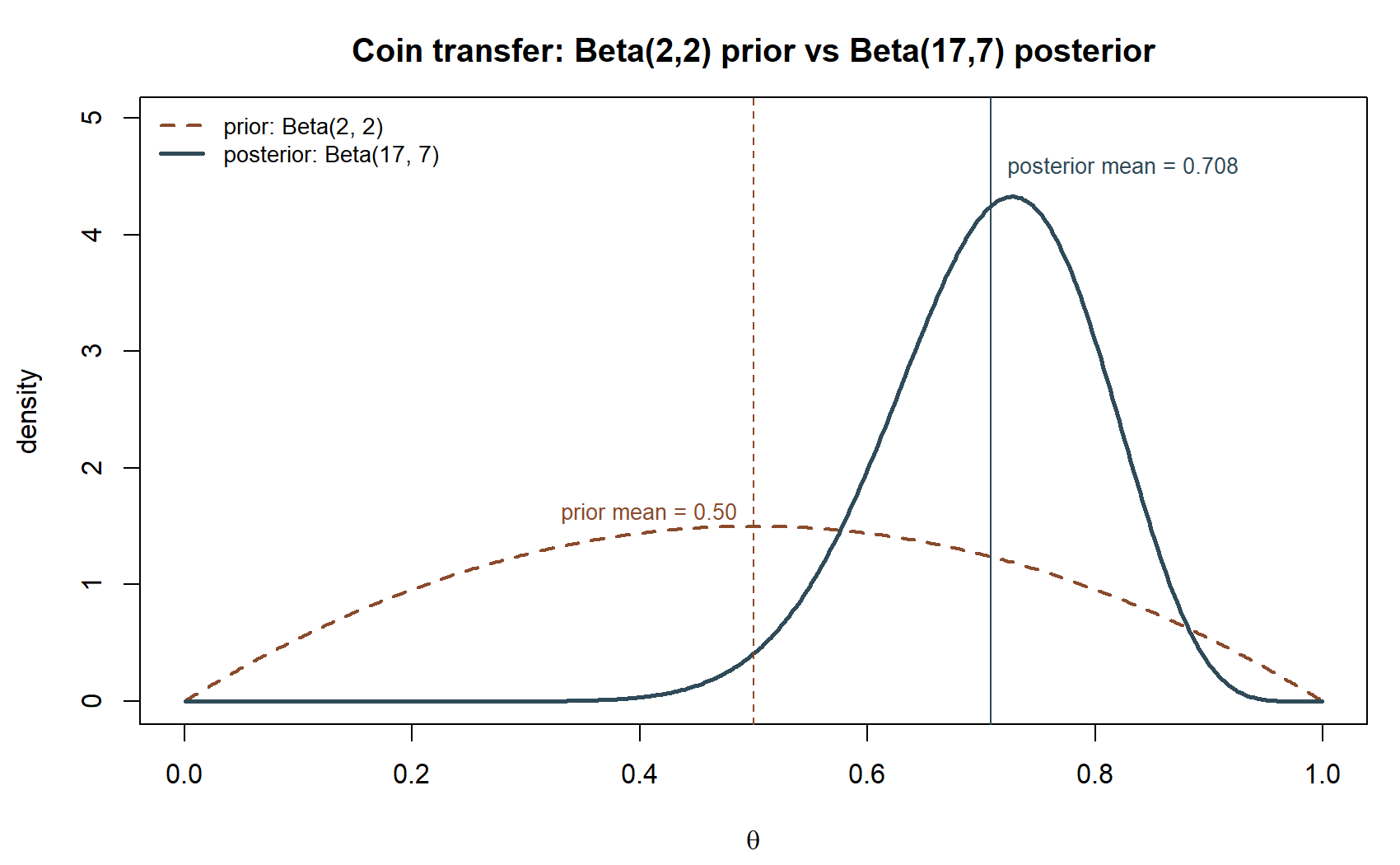
Here the weak \(\text{Beta}(2,2)\) prior (only 4 “prior flips” worth of weight) is swamped almost entirely by 20 real flips showing 15 heads — the posterior mean of \(0.708\) sits close to the raw sample proportion \(15/20 = 0.75\), pulled only slightly toward the prior’s \(0.50\). This mirrors the MAC Study case: whenever the sample size \(n\) is large relative to the prior’s implied sample size \(a+b\), the posterior is dominated by the data, and the specific prior chosen matters less. A much stronger prior (larger \(a+b\), same mean) would pull the posterior mean noticeably farther from the raw sample proportion — that sensitivity check is left to the practice problems below.
A convention warning
A credible interval and a confidence interval answer different questions, even when they use the same normal approximation and even when their numbers look similar. The Week 7 confidence interval for \(\mu\), \((44.9, 54.7)\), is a property of a repeated-sampling procedure: if the same sampling and interval-construction recipe were repeated over and over, about 95% of the resulting intervals would contain the true (fixed, unknown) \(\mu\). Any single realized interval either does or does not contain \(\mu\) — probability language does not apply to that fixed interval and fixed constant. The notation ledger’s convention-risk flag makes this explicit: a CI is not “a 95% probability the parameter is in this interval.”
The credible interval derived above, \((0.283, 0.463)\), means something different in kind, not just in degree. Because Bayesian inference treats \(\pi\) itself as a random variable with the posterior distribution \(\text{Beta}(41, 69)\), the statement “there is a 95% probability that \(\pi\) lies in \((0.283, 0.463)\)” is a direct, literal probability statement about \(\pi\) — and it is a perfectly valid statement to make, given the posterior distribution just derived. It is emphatically not the same claim a frequentist confidence interval makes, and the two should never be described with the same sentence.
That validity, though, comes with a condition that must always be stated alongside it: the credible interval’s probability statement is conditional on the prior actually used — here, \(\text{Beta}(3,7)\), the MAC director’s stated belief. A different director with a different prior, updated by the exact same survey data, would derive a different posterior and a different credible interval. The confidence interval’s guarantee, by contrast, does not depend on anyone’s prior belief at all — it depends only on the repeated-sampling behavior of the estimation procedure. Neither interval is “more correct” in general; they answer different questions under different assumptions, and this course’s pluralistic stance (§1 of the syllabus) is precisely that both are legitimate tools, so long as each is described accurately and never in the other’s language.
Practice (ungraded)
Self-check only — no submission, no key.
- Suppose the MAC director instead started with a much stronger prior, \(\text{Beta}(a=30,\, b=70)\) (same mean \(0.30\), but ten times the “prior sample size” of the \(\text{Beta}(3,7)\) used above). Using the same survey data (\(n=100\), \(k=38\)), derive the posterior distribution and its mean. Is the posterior mean closer to or farther from the raw sample proportion \(\hat\pi = 0.38\) than this week’s worked example was, and does that match the weighted-average formula derived above?
- For the coin-flip transfer example, suppose instead of \(\text{Beta}(2,2)\) the prior had been \(\text{Beta}(20,20)\) (same mean \(0.50\), much stronger). Using the same new data (\(n=20\), \(k=15\)), find the new posterior distribution and its mean. Explain in words why a stronger prior changes the answer even though the data are identical.
- In your own words, explain why the constant \(\binom{n}{k}\) can be dropped when deriving the posterior’s functional form, but the posterior still needs to be a valid probability density that integrates to 1. What step in the derivation restores that missing normalization?
Reading and source pointer
MIT OCW 18.05 covers Bayesian updating and conjugate priors, including the Beta-Binomial case, and this page’s scope, terminology, and notation level are grounded in that treatment. These notes are the course’s own synthesis, grounded in but not copied from the source.
Public vs. graded
These notes, the examples, and the practice here are public and ungraded — study material only. No graded prompts, answer keys, rubrics, point values, or due dates appear on this site. Graded inference checkpoints, quizzes, homework, labs, the midterm, the project, and the final live in Blackboard (the LMS), which is authoritative for due dates, submissions, and grades. If this page and Blackboard ever disagree, follow Blackboard.
Looking ahead
Week 13 puts every framework this course has built side by side — classical estimation and confidence intervals, likelihood and MLE, bootstrap resampling, permutation tests, and this week’s Bayesian updating — all applied to the same MAC Study usage-rate question, so the frequentist/Bayesian contrast drawn above becomes one part of a fuller comparison across all four inferential traditions.