set.seed(35103)

# Simulate the null sampling distribution: if H0: mu = 45 were exactly true,
# what would repeated sample means (n = 36, SE = 2.5) look like?
mu0 <- 45
se  <- 2.5
n_sim <- 100000

null_xbars <- rnorm(n_sim, mean = mu0, sd = se)
null_z     <- (null_xbars - mu0) / se

observed_z <- 1.92
empirical_p <- mean(abs(null_z) >= observed_z)   # "data this extreme or more, under H0"

empirical_p   # compare to the theoretical two-sided p = 0.0548

hist(null_xbars, breaks = 60, freq = FALSE,
     main = "Simulated null sample means", xlab = "simulated sample mean (minutes)")
curve(dnorm(x, mu0, se), add = TRUE)
abline(v = 49.8, lty = 1) # the observed sample mean, for comparisonWeek 8 — Hypothesis tests and p-values
Testing a claim about a parameter against the data, and reading a p-value correctly
The week question
You have a claim about a population parameter — “the average MAC visit lasts 45 minutes,” “this coin is fair” — and a sample of data. How do you turn the data into a disciplined judgment about whether the claim is credible, without ever getting to say the claim is “true” or “false” with certainty? That is the job of a hypothesis test, and the number at its center — the p-value — is one of the most quoted and most misread numbers in all of statistics. This week builds the test from its pieces (null and alternative hypotheses, a test statistic, a p-value) and is deliberately blunt about what a p-value is not.
Why this matters
Hypothesis testing is the machinery behind an enormous share of applied claims: does a new teaching method raise scores, does a drug beat placebo, does a website redesign change click-through rate. Every one of these claims eventually gets compressed into a p-value that someone reports in a paper, a press release, or a meeting. If you cannot read that number correctly, you cannot evaluate the claim behind it. Weeks 1 through 7 built the vocabulary of parameters, sampling distributions, and confidence intervals. This week turns that machinery around: instead of estimating a parameter, you use the same sampling-distribution logic to weigh evidence against a specific stipulated value of that parameter.
Learning goals
By the end of this week, you should be able to:
- State a null hypothesis \(H_0\) and an alternative hypothesis \(H_a\) for a claim about a mean or a proportion.
- Build the test statistic that measures how far the sample statistic falls from the null value, in standard-error units.
- Define the p-value precisely as \(P(\text{data this extreme or more} \mid H_0 \text{ true})\), and explain in your own words why this is not \(P(H_0 \text{ true})\).
- Compare a p-value to a chosen significance level \(\alpha\) and state a decision (“reject \(H_0\)” or “fail to reject \(H_0\)”) without overstating what that decision means.
- Recognize a borderline result for what it is: neither strong evidence against \(H_0\) nor proof that \(H_0\) is correct.
Core vocabulary
- Null hypothesis (\(H_0\)). A specific, stipulated claim about the parameter — the “status quo” or “nothing interesting is happening” position, stated as an equality (for example \(H_0: \mu = 45\)).
- Alternative hypothesis (\(H_a\)). The claim you would consider instead if the data give strong enough evidence against \(H_0\) — here two-sided (\(H_a: \mu \neq 45\)), meaning you would be interested in a difference in either direction.
- Test statistic. A standardized measure of how far the sample statistic is from the null value, in standard-error units — here \(z = (\bar{x} - \mu_0)/\mathrm{SE}(\bar{x})\).
- p-value. \(P(\text{data this extreme or more extreme} \mid H_0 \text{ true})\) — the probability, computed under the assumption that \(H_0\) is exactly true, of seeing a test statistic at least as far from 0 as the one you actually got.
- Significance level (\(\alpha\)). A threshold chosen before looking at the data (conventionally 0.05), against which the p-value is compared to reach a decision.
- Reject / fail to reject \(H_0\). The two possible decisions. “Fail to reject” is not the same as “accept” or “prove” — it means the data did not give strong enough evidence against \(H_0\) at the chosen \(\alpha\).
Concept development
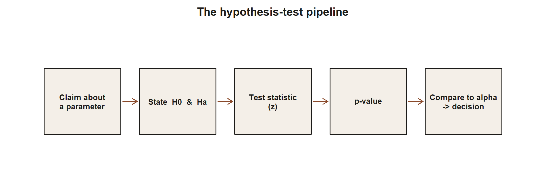
Every hypothesis test in this course follows the same five-step pipeline, no matter whether the claim is about a mean, a proportion, or something else. The rest of this section builds each step in turn; keep this picture in mind as the anchor.
From confidence intervals to hypothesis tests
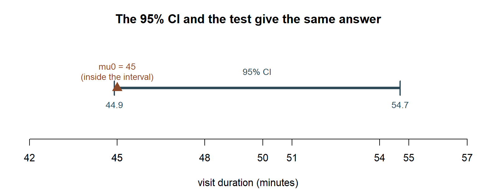
Week 7 built a confidence interval: a range of plausible values for a parameter, built entirely from the sample. A hypothesis test asks almost the same question from the other direction. Instead of “what range of values is plausible for \(\mu\),” it asks “is this one specific, stipulated value of \(\mu\) plausible, given what I observed?” Both procedures use the same sampling-distribution machinery — the same standard error, the same normal (or \(t\)) shape — just aimed at a different question. In fact, for a two-sided test at level \(\alpha = 0.05\), the null value is rejected exactly when it falls outside the 95% confidence interval. The two tools are two views of the same underlying logic, not two unrelated ideas.
Setting up the two hypotheses
Every hypothesis test starts with a pair of competing claims about a population parameter, written before any data are examined:
\[H_0: \theta = \theta_0 \qquad \text{vs.} \qquad H_a: \theta \neq \theta_0\]
\(H_0\) names one specific stipulated value \(\theta_0\) for the parameter — never a range. \(H_a\) here is two-sided: it says the true parameter differs from \(\theta_0\), without committing to a direction. (A one-sided alternative, \(H_a: \theta > \theta_0\) or \(H_a: \theta < \theta_0\), is possible when there is a specific directional question in view — Week 9 uses a one-sided setup for a power calculation — but the default, and the one used in this week’s worked example, is two-sided.) The choice of \(H_0\) and \(H_a\) is a scientific and practical decision, made before the data are collected or examined; it is not something you get to adjust after seeing which way the data happen to point.
Building the test statistic
Once \(H_0\) names a specific value \(\theta_0\), the sampling distribution of the sample statistic under \(H_0\) is known (or approximated) — this is exactly the sampling-distribution machinery from Week 2 and Week 3, just centered at the null value instead of at the unknown true parameter. The test statistic measures how many standard errors the observed sample statistic sits away from that null value:
\[z = \frac{\bar{x} - \mu_0}{\mathrm{SE}(\bar{x})}\]
for a test about a mean with known \(\sigma\) (the same known-\(\sigma\) teaching simplification used since Week 2), or, for a test about a proportion,
\[z = \frac{\hat{p} - \pi_0}{\mathrm{SE}(\hat{p})}, \qquad \mathrm{SE}(\hat{p}) = \sqrt{\frac{\pi_0(1-\pi_0)}{n}}.\]
Large \(|z|\) means the sample statistic is many standard errors from the null value — data that would be surprising if \(H_0\) were really true. Small \(|z|\) means the sample statistic is close to the null value — data that look perfectly ordinary under \(H_0\).
From test statistic to p-value, and the decision rule
The p-value converts the test statistic into a probability, using the sampling distribution assumed under \(H_0\):
\[p = P(\text{a test statistic at least as extreme as the observed one} \mid H_0 \text{ true}).\]
For a two-sided test using the standard normal reference distribution, this is \(p = 2 \times P(Z > |z|) = 2\left(1 - \Phi(|z|)\right)\), where \(\Phi(\cdot)\) is the standard normal cdf: the factor of 2 accounts for the two-sided alternative, since either a large positive or a large negative \(z\) counts as evidence against \(H_0\). Once you have the p-value, the decision rule is mechanical: compare \(p\) to the chosen \(\alpha\). If \(p \le \alpha\), reject \(H_0\) in favor of \(H_a\) — the data are unusual enough under \(H_0\) that you no longer find \(H_0\) credible. If \(p > \alpha\), fail to reject \(H_0\) — the data are not unusual enough, under \(H_0\), to abandon it. Neither decision proves anything; both are calibrated statements about how surprising the data would be if \(H_0\) were exactly true.
Worked examples
Worked example — Is last year’s average visit duration still right? (the MAC Study)
Setup, symbolically. Last year’s campus baseline average MAC visit duration was \(\mu_0 = 45\) minutes. This term’s research team wants to know whether the average has changed, so they set up a two-sided test:
\[H_0: \mu = 45 \qquad \text{vs.} \qquad H_a: \mu \neq 45.\]
They use this week’s visit-duration sample: \(n = 36\), \(\bar{x} = 49.8\) minutes, with the known-\(\sigma\) teaching simplification \(\sigma \approx 15\) carried since Week 2, giving \(\mathrm{SE}(\bar{x}) = \sigma/\sqrt{n} = 15/6 = 2.5\). The test statistic is
\[z = \frac{\bar{x} - \mu_0}{\mathrm{SE}(\bar{x})} = \frac{49.8 - 45}{2.5} = \frac{4.8}{2.5} = 1.92.\]
Numerically, the p-value. For a two-sided test, \(p = 2(1 - \Phi(1.92))\). Standard normal tables (or software) give \(\Phi(1.92) \approx 0.9726\), so \(1 - \Phi(1.92) \approx 0.0274\), and
\[p = 2(0.0274) = 0.0548.\]
Seeing it. Before reading the result in words, look at where 49.8 actually falls under the null curve, and what “the p-value” looks like as a picture rather than a formula output.
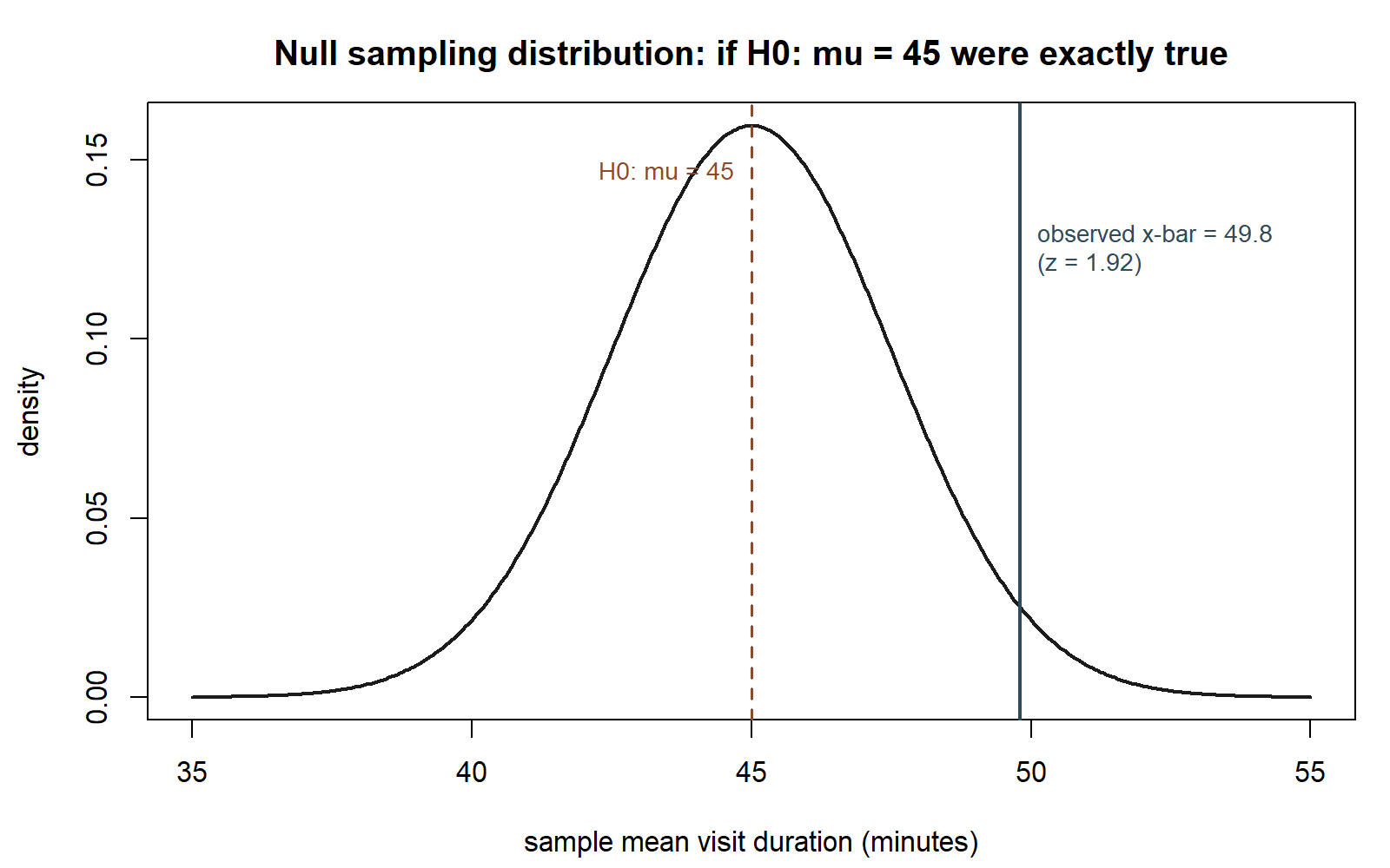
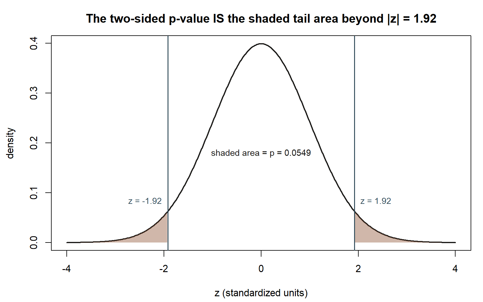
Reading the result. At the conventional \(\alpha = 0.05\), this p-value of about 0.0548 is just above \(\alpha\): the team fails to reject \(H_0: \mu = 45\), but only just. This is a deliberately borderline case, and it is worth sitting with what that does and does not mean:
- It does not mean the average visit duration is 45 minutes, or that the sample mean of 49.8 is “wrong.” The sample gave real evidence pointing away from 45 — just not quite enough, by the \(\alpha = 0.05\) yardstick, to call it conclusive under this framework.
- It does not mean \(H_0\) has been shown to be true or even “likely true.” Failing to reject is a statement about insufficient evidence to abandon \(H_0\), not a certification of \(H_0\).
- A different, only slightly larger sample, or a slightly larger observed gap, could easily have pushed \(p\) below 0.05. The result is sensitive to exactly this kind of borderline; that sensitivity is a feature of what a fixed threshold like \(\alpha = 0.05\) does at the edge, not a flaw specific to this dataset.
- The confidence interval from Week 7, \((44.9, 54.7)\), is consistent with this: it very narrowly contains 45 (barely, since 44.9 is only 0.1 below 45), which lines up exactly with “fails to reject \(H_0: \mu=45\) at \(\alpha = 0.05\), but only just.”
The honest summary a researcher should write here is something like: “the data show a visit-duration average somewhat above last year’s baseline, but the evidence against the baseline value is not strong enough, at the conventional 5% threshold, to declare a change with confidence.” That is a much more carefully hedged statement than either “nothing changed” or “the average has definitely gone up” — and that hedging is the point of reporting a p-value rather than a bare yes/no.
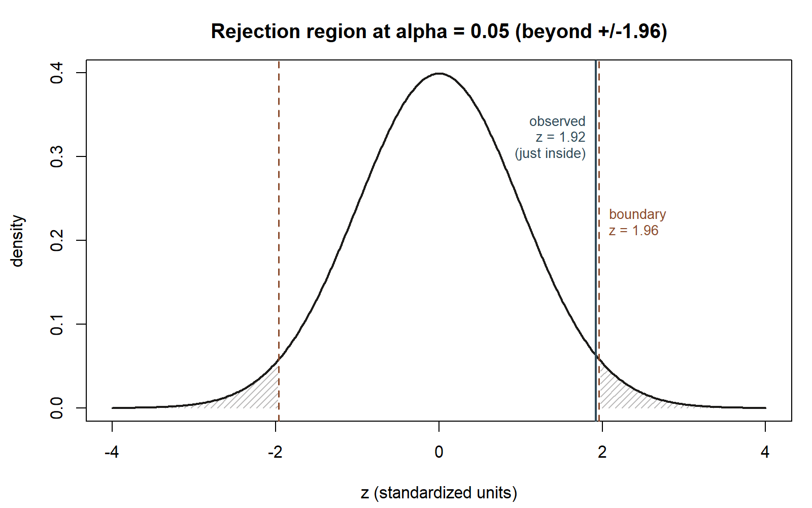
Table — reading “data this extreme or more” directly. A p-value is a tail-area statement: the fraction of the null sampling distribution at least as far from \(\mu_0\) as what was observed. The table below is the numeric companion to the two figures above — it puts a number on every distance the shaded-tail and rejection-region pictures only showed for \(z=1.92\) and \(z=1.96\) — and marks where the observed result sits relative to a few reference distances, all measured under the assumption \(H_0: \mu = 45\) is exactly true:
| Distance from \(\mu_0 = 45\), in \(SE\) units | Two-sided tail area (p-value) | Reject at \(\alpha = 0.05\)? |
|---|---|---|
| \(z = 1.00\) | \(2(1-\Phi(1.00)) \approx 0.317\) | no |
| \(z = 1.50\) | \(2(1-\Phi(1.50)) \approx 0.134\) | no |
| \(z = 1.92\) (the observed result) | \(2(1-\Phi(1.92)) \approx 0.0548\) | no, but only just |
| \(z = 1.96\) | \(2(1-\Phi(1.96)) = 0.050\) | exactly at the boundary |
| \(z = 2.50\) | \(2(1-\Phi(2.50)) \approx 0.012\) | yes |
Reading down the table shows the p-value shrinking as the observed result sits farther out in the tail of the null distribution — the observed \(z = 1.92\) falls just short of the \(z = 1.96\) boundary a two-sided \(\alpha = 0.05\) test draws.
The same idea can be seen by simulation instead of by table lookup: repeatedly generate sample means as if \(H_0\) were exactly true, and directly count how often a result at least as extreme as the one observed comes up just by chance.
This chunk is shown but not executed on this page (eval: false) — running it yourself is the point, and the prediction prompt above asked you to guess its shape and its empirical_p before you look. The figure below was produced by running exactly this simulation separately (same seed, same n_sim), so you can check your prediction against a real result:
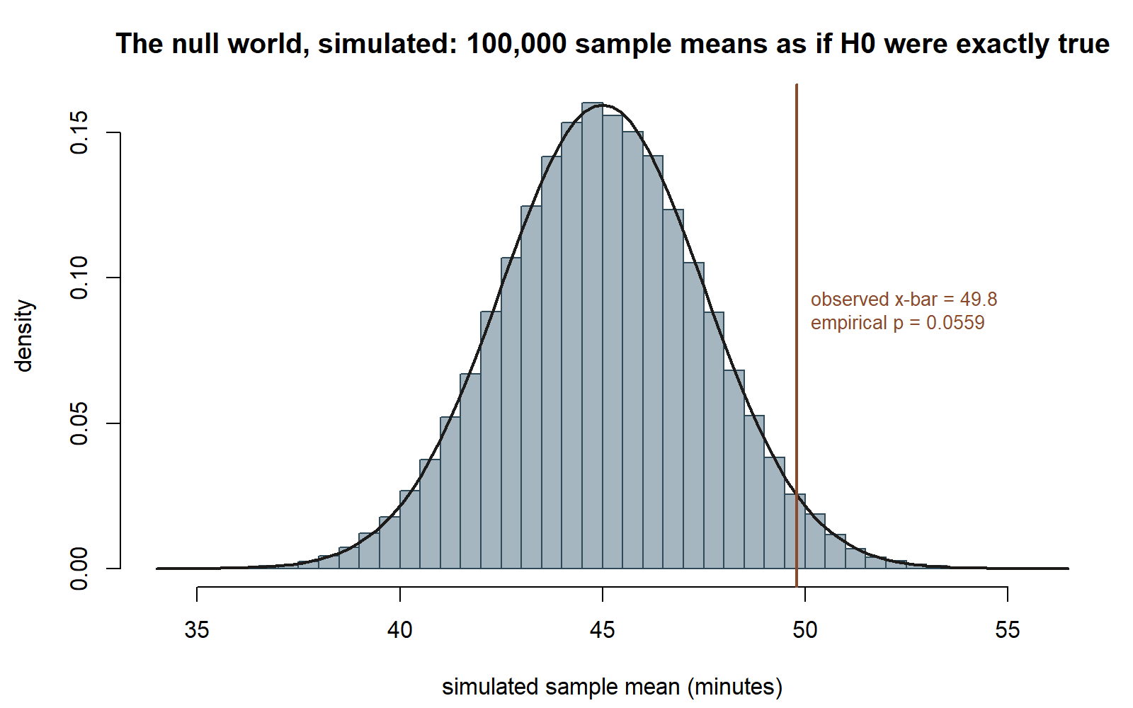
What this shows: among 100,000 simulated sample means generated as if \(\mu = 45\) were exactly true, the fraction landing at least \(1.92\) standard errors from 45 (in either direction) is \(0.0559\) — close to, though not identical to, the theoretical p-value of \(0.0548\) (simulation is itself random; a different seed or a different n_sim gives a slightly different empirical value). This is the p-value’s definition made concrete: not a probability that \(H_0\) is true, but the fraction of a purely-hypothetical null world that would look at least this extreme. Synthetic instructional example; numbers are illustrative.
Worked example — is this coin fair? (transfer example; synthetic)
Context (synthetic). Suppose a friend hands you a coin and claims it is fair. You flip it \(n = 100\) times (synthetic data, not the MAC Study) and observe \(k = 58\) heads, so \(\hat{p} = 58/100 = 0.58\). You want to test whether this is consistent with a fair coin.
Setup, symbolically.
\[H_0: \pi = 0.5 \qquad \text{vs.} \qquad H_a: \pi \neq 0.5,\]
where \(\pi\) is the true long-run probability the coin lands heads. Under \(H_0\), the standard error of \(\hat{p}\) is
\[\mathrm{SE}(\hat{p}) = \sqrt{\frac{\pi_0(1-\pi_0)}{n}} = \sqrt{\frac{0.5 \times 0.5}{100}} = \sqrt{0.0025} = 0.05.\]
Numerically. The test statistic is
\[z = \frac{\hat{p} - \pi_0}{\mathrm{SE}(\hat{p})} = \frac{0.58 - 0.50}{0.05} = \frac{0.08}{0.05} = 1.60.\]
The two-sided p-value is \(p = 2(1 - \Phi(1.60))\). Since \(\Phi(1.60) \approx 0.9452\), this gives \(p \approx 2(0.0548) = 0.1096\). At \(\alpha = 0.05\), \(p \approx 0.11 > 0.05\), so you fail to reject \(H_0: \pi = 0.5\): 58 heads out of 100 flips is not unusual enough, under the assumption of a fair coin, to conclude the coin is biased.
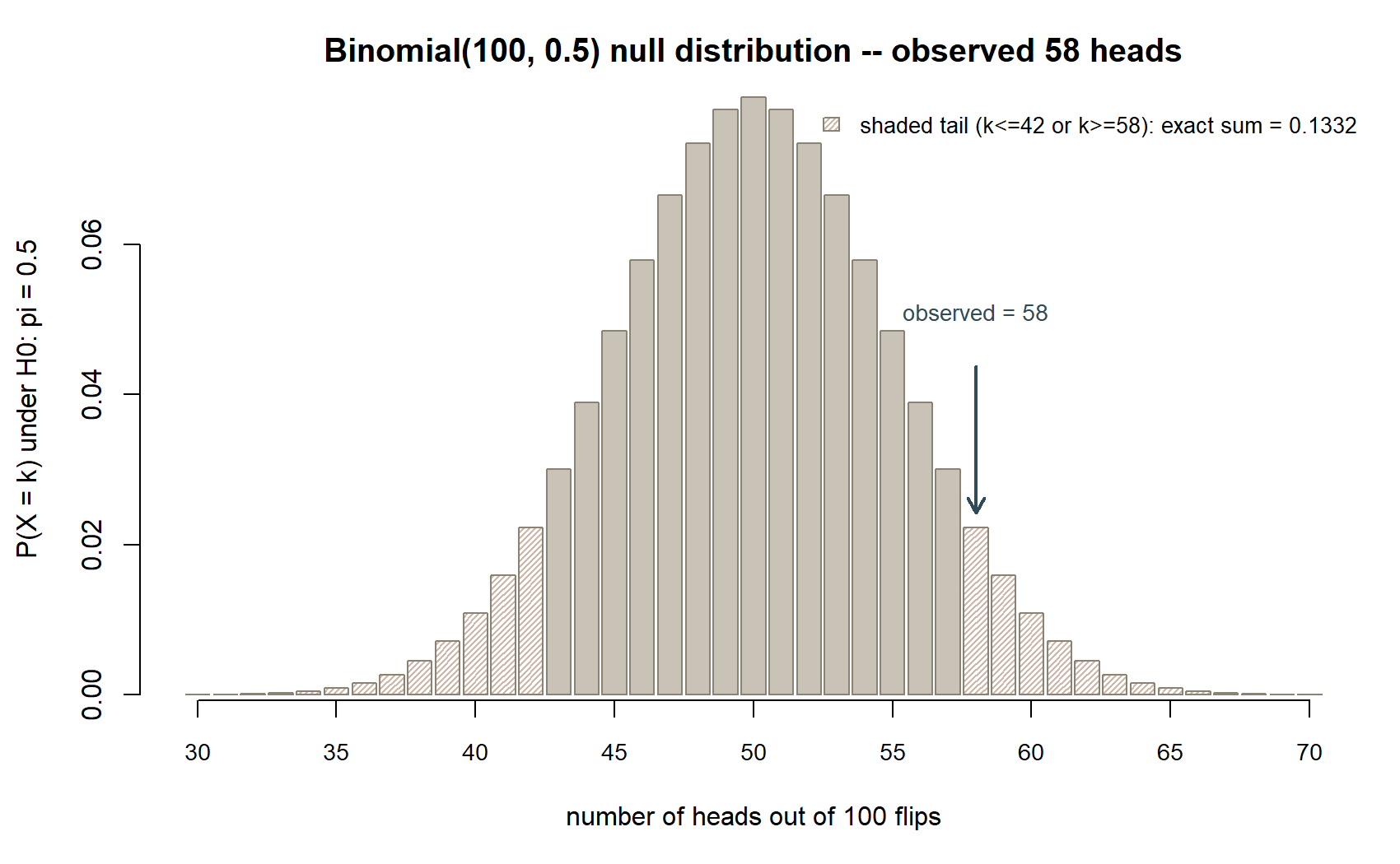
This example gets its own null distribution — a discrete one, since a head count can only take whole-number values, unlike the continuous curve the MAC study used.
Naming the classic misinterpretation directly. It is extremely tempting to read \(p \approx 0.11\) as “there is an 11% chance the coin is fair,” or its mirror image, “there is an 89% chance the coin is biased.” Both readings are wrong, and this is the single most common misinterpretation of a p-value. The p-value is not a probability statement about \(H_0\) at all — \(H_0\) is either true or it is not, and the p-value does not update a probability attached to it. The p-value is a probability statement about the data, computed under the assumption that \(H_0\) is exactly true:
\[p = P(\text{data this extreme or more extreme} \mid H_0 \text{ true}) \;\;\neq\;\; P(H_0 \text{ true}).\]
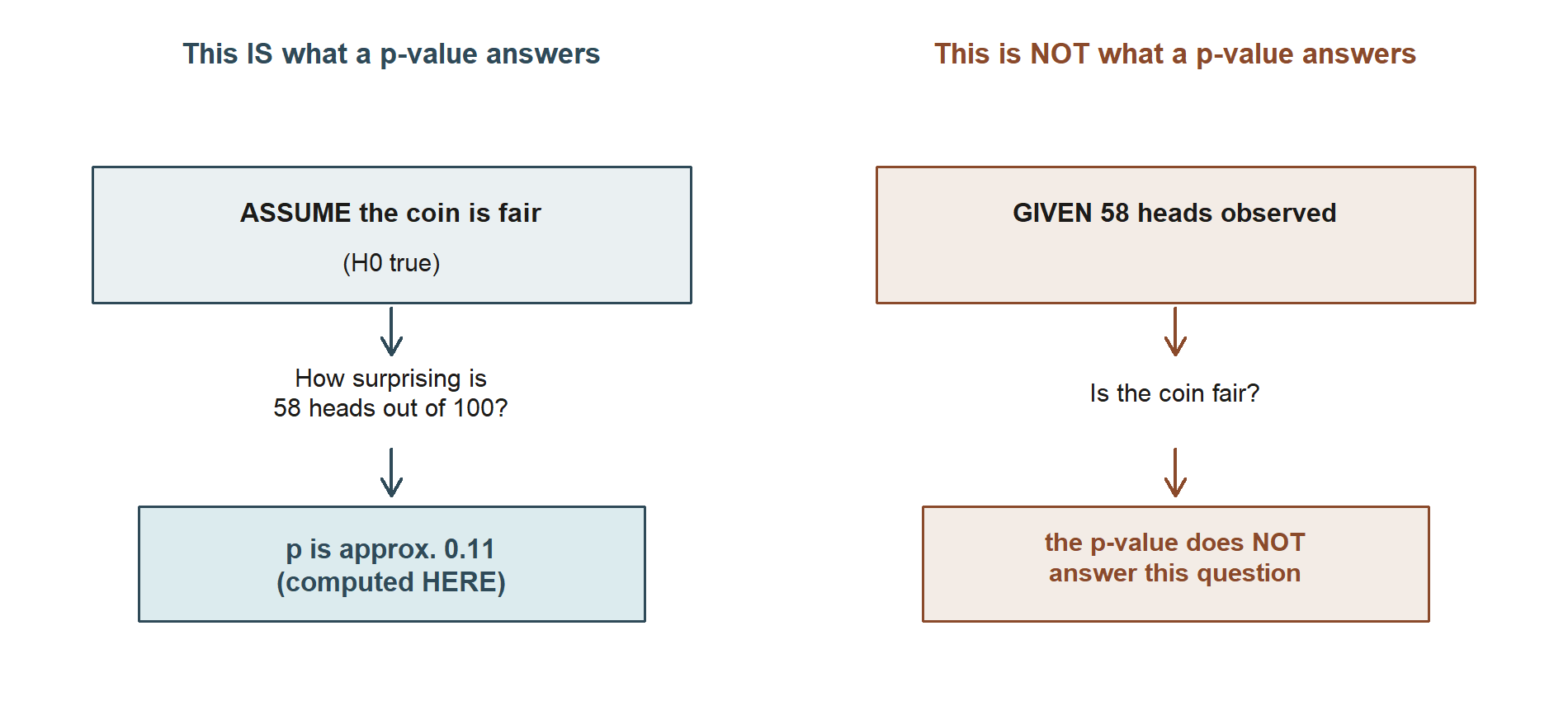
Concretely: \(p \approx 0.11\) means “if this coin really were exactly fair, you would see a result at least as far from 50 heads as 58 heads (that is, 58 or more, or 42 or fewer) about 11% of the time, just from ordinary flip-to-flip variability.” It says nothing about the probability that the coin is fair, because the coin’s fairness is a fixed fact, not a random quantity with a probability attached in this framework.
A common mistake
The p-value is not \(P(H_0 \text{ true})\), and a small p-value does not mean “\(H_0\) is probably false.” This is convention-risk flag #1 for the course, and it deserves to be stated as bluntly as possible: a p-value is computed by assuming \(H_0\) is true and then asking how surprising the observed data would be under that assumption. It is a statement about the data, conditional on \(H_0\) — never a statement about the probability that \(H_0\) itself is true or false. Two closely related mistakes to watch for:
- Treating “fail to reject \(H_0\)” as “\(H_0\) is proven true” or “there is no effect.” It only means the evidence against \(H_0\) was not strong enough at the chosen \(\alpha\) — as the borderline MAC-Study result above illustrates directly.
- Treating \(\alpha = 0.05\) as a sharp line between “real” and “not real.” A p-value of 0.048 and a p-value of 0.055 reflect nearly identical strength of evidence; the decision rule draws a bright line through data that do not actually change that abruptly.
Low-stakes self-checks (ungraded)
These are practice only — ungraded, self-check prompts to test your own understanding before moving on.
- Write out \(H_0\) and \(H_a\) for a two-sided test of whether the MAC’s average visit duration differs from 45 minutes. Which of the two hypotheses names a single specific value?
- Using \(\bar{x} = 49.8\), \(\mu_0 = 45\), and \(\mathrm{SE}(\bar{x}) = 2.5\), recompute the test statistic \(z\) by hand and check it against the worked example above.
- In your own words, explain why \(p \approx 0.0548\) is not “a 5.48% chance the true average is 45 minutes.”
- For the coin example, if the observed p-value had been 0.03 instead of about 0.11, would the decision at \(\alpha = 0.05\) change? Would the meaning of the p-value (as a conditional probability about the data) change?
- Explain, in one or two sentences, why “fail to reject \(H_0\)” is a weaker and more careful statement than “\(H_0\) is true.”
Reading and source pointer
This week’s core framework — setting up null and alternative hypotheses, building a test statistic, and computing a p-value under the null — follows the hypothesis-testing and p-values material in MIT OCW 18.05, Introduction to Probability and Statistics. Because this week’s center is genuinely hypothesis-testing practice, it also draws on the hypothesis-testing chapter of Statistical Inference via Data Science: A ModernDive into R and the Tidyverse (2nd ed., Ismay, Kim, Valdivia), which frames a p-value in terms of a simulated null distribution — a framing described here in words, with the equivalent computation always shown in base R rather than ModernDive’s infer pipeline (per the course’s house-style adaptation). These notes are the course’s own synthesis, grounded in but not copied from the sources.
Public vs. graded
These notes, the examples, and the practice here are public and ungraded — study material only. No graded prompts, answer keys, rubrics, point values, or due dates appear on this site. Graded inference checkpoints, quizzes, homework, labs, the midterm, the project, and the final live in Blackboard (the LMS), which is authoritative for due dates, submissions, and grades. If this page and Blackboard ever disagree, follow Blackboard.
Looking ahead
A test result is not the whole story: every test can go wrong in one of two ways (rejecting a true \(H_0\), or failing to reject a false one), and the chance of each kind of error depends on choices you make before collecting data. Week 9 makes this precise — Type I and Type II error, statistical power, and the trade-offs behind choosing \(\alpha\) and a sample size — using this same visit-duration setup, now asking “how likely would this test have been to catch a real change of a given size?”
See also
- Week 7 — Confidence intervals (+ midterm) — the same sampling-distribution machinery, aimed at estimating a range instead of testing a stipulated value.
- Week 9 — Error rates, power, and decisions — what can go wrong with a test, and how to quantify it.
- Resources — Notation glossary
- Resources — Inference formula reference