Week 13 — Comparing inferential frameworks

The same question, the same data, four different machines for answering it

The week question

Over the last twelve weeks you have built four genuinely different machines for turning a sample into a statement about an unknown parameter: maximum likelihood estimation (Weeks 5–6), the classical frequentist confidence interval (Week 7), the bootstrap (Week 10), and Bayesian posterior inference (Week 12). Each of these machines, pointed at the same question — what is the population proportion π of students who use the MAC in a given week? — produces a number, or a range of numbers, that look reassuringly similar. This week’s question is not “which machine is right?” (this course does not declare a winner). It is: when you line up all four answers side by side, where do they agree, where do they diverge, and — the harder and more important question — what does each one actually claim, even in the cases where the numbers coincide?

Why this matters

It is tempting, once you have four numbers that are all close to 0.38, to treat them as interchangeable — different paths to the “same” answer, so the differences between the frameworks must be bookkeeping. That temptation is exactly the trap this week exists to dismantle. A confidence interval, a bootstrap interval, and a credible interval can be numerically almost identical while asserting three logically distinct things about what “95%” refers to. Knowing which framework you are using — and being able to say precisely what its output does and does not claim — is arguably the single most transferable skill of an inference course, because in practice you will read papers and software output that mix all four idioms freely, often without labeling which one is in play. This week is the payoff for keeping “likelihood,” “confidence,” and “posterior” visually and verbally distinct all term — now you see all three side by side and watch that discipline earn its keep.

Learning goals

By the end of this week you should be able to:

Assemble a single side-by-side comparison of a point estimate and an interval for the same parameter (the MAC Study usage rate π) under all four frameworks studied this term.
State, without hedging, what each framework’s interval formally claims — a confidence interval, a bootstrap interval, and a credible interval do not all claim the same thing, even when their numbers overlap.
Explain why the frequentist CI and the Bayesian credible interval are numerically close in this particular case (a comparatively weak prior relative to a moderately large sample), and recognize that this closeness is a feature of this specific example, not a general law.
Identify what each framework needs as an input that the others do not (a stipulated model and fixed data for likelihood; a repeated-sampling story for the frequentist CI; resampling of the observed data for the bootstrap; a prior distribution for the Bayesian posterior).
Choose, given a new applied question, which framework’s claim is the one you actually want to make — and say why the other three would answer a different question.

Core vocabulary

Point estimate. A single best-guess number for an unknown parameter, computed from the sample data — π̂ = 0.38 in the MLE and frequentist framings, or the posterior mean ≈ 0.373 in the Bayesian framing. Every framework produces one, but they do not always mean the same thing even when they are numerically close.
Confidence interval (CI) — recap. A range built so that the procedure captures the true parameter a stated percentage of the time over hypothetical repeated sampling (Week 7). A property of the method, not a probability statement about one already-computed interval.
Bootstrap interval — recap. A range built by resampling the observed data with replacement many times and reading percentiles off the resulting distribution of estimates (Week 10). Answers the same kind of repeated-sampling question as the classical CI, but estimates the sampling variability directly from the data rather than from a normal-theory formula.
Credible interval — recap. A range of parameter values that the posterior distribution assigns a stated probability of containing the parameter, conditional on the prior and the observed data (Week 12). Unlike a CI, this is a genuine probability statement about the parameter itself, since the parameter now has its own probability distribution (the prior, updated to the posterior).
Framework. A complete way of turning data (and, for the Bayesian case, a prior) into a statement about a parameter — this week treats maximum likelihood, frequentist, bootstrap, and Bayesian as four such frameworks, all legitimate, none declared uniquely correct by this course.

Concept development

Setting up a fair comparison

To compare frameworks honestly, you need to hold the question and the data fixed and vary only the machine. This week reuses a single thread that has run since Week 3: the MAC usage-rate survey, in which n = 100 students were asked whether they used the MAC at least once in a given week, and k = 38 said yes. That single dataset is the input to three of the four rows in the table below; the fourth (the MLE) uses this same full survey for its point estimate, but the pilot MLE derivation in Weeks 5–6 was actually carried out on a smaller illustrative batch, which is itself worth re-examining as a comparison point. Holding the data fixed like this is what makes the comparison meaningful — if both the data and the method varied, any difference in the answers could be attributed to either cause, and the comparison would teach you nothing about the methods themselves.

Four rows, one parameter

The table below lines up all four frameworks’ treatment of the MAC usage rate π. Read down the “point estimate” column first, then across each row for what the interval claims.

Framework	Point estimate	Interval / range	What the interval formally claims
Maximum likelihood (Wks 5–6)	π̂ = k/n	(no interval derived; MLE gives a point estimate, not a range, in this course’s treatment)	The single value of π that makes the observed data most likely, among all possible values — a comparison-based, not a probability, claim
Frequentist (Wk 7)	p̂ = 0.38	(0.285, 0.475)	A range built by a procedure that, applied over many hypothetical repeated samples of size n = 100, would contain the true π 95% of the time
Bootstrap (Wk 10)	p̂ = 0.38	qualitatively similar range (see below)	A range built by resampling the observed 100 responses with replacement many times; estimates the same kind of repeated-sampling coverage as the frequentist CI, but from the data’s own resampled variability rather than a normal-theory formula
Bayesian (Wk 12)	posterior mean ≈ 0.373	(0.283, 0.463)	A range that the posterior distribution assigns a 95% probability of containing π, given the Beta(3, 7) prior and the observed data

Two more numbers are worth naming explicitly even though they are not full framework rows on their own: the small pilot MLE, π̂ = 2/5 = 0.4 (Weeks 5–6), and the raw sample proportion from the full survey, p̂ = 38/100 = 0.38 (used from Week 3 onward). These two numbers differ — 0.4 versus 0.38 — and the reason is not a disagreement about method; it is a difference in sample size. The pilot MLE was deliberately computed from just n = 5 responses (kept small on purpose so the likelihood arithmetic could be done by hand), while the frequentist, bootstrap, and Bayesian rows above all use the full n = 100 survey. A smaller sample produces a noisier estimate — 2 successes out of 5 gives exactly 0.4, but that same underlying process, sampled 100 times instead of 5, happened to produce 38 successes, or p̂ = 0.38. Both are legitimate maximum likelihood estimates of π for the sample each was computed from — their difference is a sample-size story, not a methods story.

Where the frameworks agree, and why

Look specifically at the frequentist CI, (0.285, 0.475), and the Bayesian 95% credible interval, (0.283, 0.463). These two ranges nearly overlap — both centered in the high-0.3s / low-0.4s, with similar widths (about 0.19 versus about 0.18). This closeness is not a coincidence, but it is also not a general law; it happens here because of a specific balance between the prior and the data.

The prior used in Week 12, Beta(a = 3, b = 7), carries a prior mean of 3/10 = 0.30 and an effective sample size, in the sense that matters for a Beta-Binomial update, of only a + b = 10 “pseudo-observations.” The actual survey contributes n = 100 real observations — ten times as much information as the prior encodes. When a weak prior is updated by substantially more data than the prior itself represents, the data dominate the posterior, and the posterior mean drifts close to the data’s own estimate (the posterior mean of Beta(41, 69) is 41/110 ≈ 0.373, much closer to the sample p̂ = 0.38 than to the prior mean of 0.30); the posterior’s spread likewise comes to resemble the frequentist sampling-variability calculation, because both are driven mostly by the same n = 100 observations rather than by the prior’s shape.

Had the prior instead been sharply concentrated and/or built from many more pseudo-observations — say, a prior like Beta(300, 700), representing strong prior conviction backed by the equivalent of 1,000 pseudo-observations — the posterior would have stayed close to the prior’s belief even after seeing the n = 100 survey, and the Bayesian credible interval could have looked quite different from the frequentist CI, centered closer to 0.30 rather than to 0.38. The lesson is general: a weak prior relative to the sample size lets a Bayesian answer converge toward the frequentist answer; a strong prior does not — and you can check which situation you are in by comparing a + b (the prior’s pseudo-sample size) against n (the data’s actual sample size).

Where the frameworks differ in what they claim — even when the numbers agree

This is the more important half of the comparison, and it is easy to let it slide once the numbers look alike. Even though (0.285, 0.475) and (0.283, 0.463) are numerically close, they answer two different questions, in two different grammars. The frequentist CI says: “we used a procedure that, if we imagine repeating this n = 100 survey over and over, would produce an interval containing the true π in 95% of those hypothetical repetitions.” Before the data are collected, the interval’s endpoints are the random quantities; π itself is treated as a fixed, if unknown, constant. Once the specific interval (0.285, 0.475) is computed, it either does or does not contain the true π — there is no probability left to assign to that already-settled fact (exactly the Week 7 warning against saying “there’s a 95% probability π is in this interval”). The credible interval says something a frequentist framework is formally not allowed to say: “given the Beta(3, 7) prior and the observed data, there is a 95% probability that π itself lies in (0.283, 0.463).” Here π is treated as a random quantity with its own probability distribution (the posterior), so a direct probability statement about π’s location is licensed — but only relative to the stated prior. Change the prior, and the credible interval changes; there is no prior-free Bayesian answer.

The two claims are easiest to tell apart side by side, as two separate chains of reasoning rather than two readings of one picture:

Two labeled panels. The left panel, titled what the 95 percent confidence interval claims, reads: repeat the survey many times and build the interval the same way each time; about 95 percent of those intervals would contain the true pi; this one interval, 0.285 to 0.475, either contains pi or it does not, so no probability is left to assign. The right panel, titled what the 95 percent credible interval claims, reads: combine the Beta 3,7 prior with the observed data; posterior Beta 41,69 is a probability distribution over pi itself; the probability that pi is in 0.283 to 0.463 equals 0.95, a direct probability statement about pi, valid only given the stated prior. — Figure 1: **Two different claims about “95%” (synthetic).** The confidence interval’s claim (left) lives entirely in the behavior of a repeated procedure, before any specific interval is computed; the credible interval’s claim (right) is a direct probability statement about π itself, licensed only because the posterior treats π as a random quantity. Both use the same “95%,” but the two chains of reasoning never meet.

What the figure shows (non-visual equivalent). The left chain never assigns a probability to π or to any one already-computed interval — its “95%” describes the procedure across hypothetical repeated samples. The right chain assigns a probability directly to π, because the posterior makes π a random quantity — but that statement is conditional on the Beta(3, 7) prior stated in the top box. Reading the left box’s “95%” as if it meant the right box’s claim (or vice versa) is exactly the error this week is built to prevent. Synthetic instructional example; numbers are illustrative.

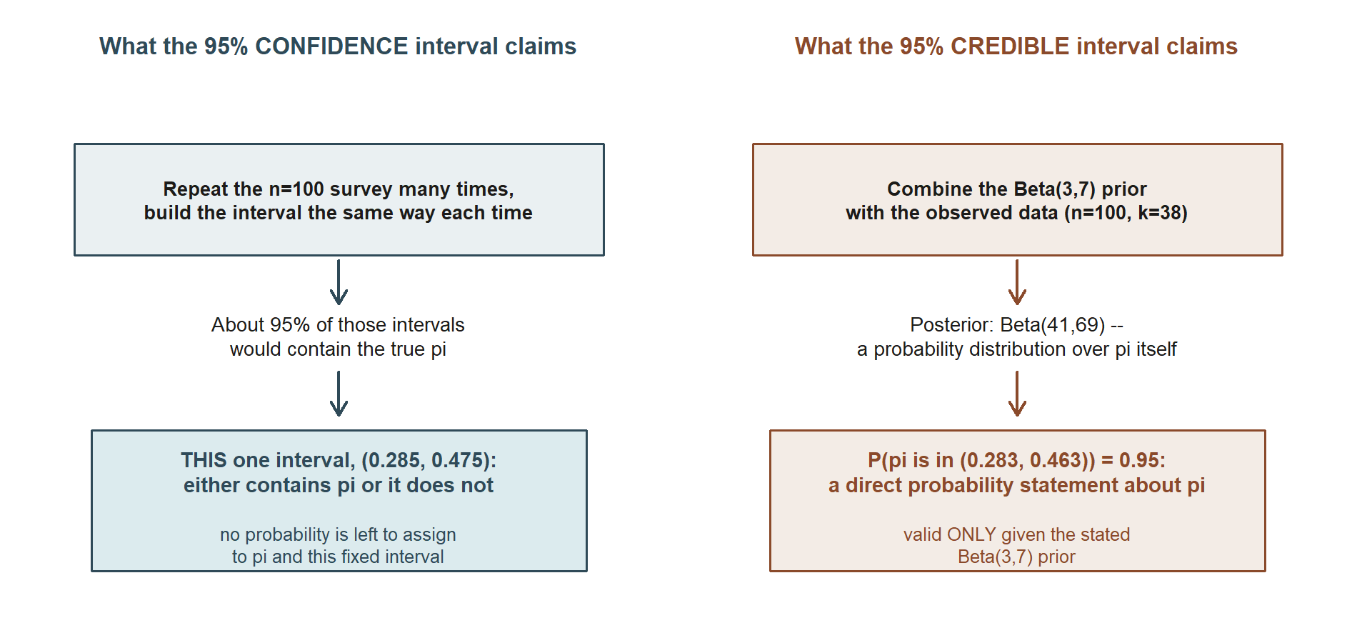
So the two intervals can be numerically close while making claims that live in different logical categories: one is a statement about the long-run behavior of a procedure, the other is a direct probability statement about the parameter, conditional on a stated prior. Mixing them up — reading a CI as if it made the credible-interval claim, or presenting a credible interval as if it needed no prior — is the single most consequential error this week is designed to prevent, and it is exactly the error that Weeks 7 and 12 separately warned against and that this week puts side by side so the contrast is unavoidable.

Table — the framework comparison matrix. The prose above walks through five separate distinctions between the frequentist and Bayesian machinery; the table below crystallizes those same five distinctions into one reference grid, dimension by dimension, so the contrast can be checked at a glance rather than re-derived from prose each time:

Dimension	Frequentist CI (and the bootstrap, which shares its logic)	Bayesian credible interval
What is treated as random	The interval’s endpoints, across hypothetical repeated samples; π is a fixed, unknown constant	π itself, via its posterior distribution; the prior and observed data are fixed once the update is done
What “95%” refers to	The long-run success rate of the interval-construction procedure, across repeated sampling	The posterior probability that π lies in this specific interval, given the prior and the data
Is “95% probability” licensed for one already-computed interval?	No — the interval either contains π or it does not; no probability is left to assign to that settled fact	Yes — π has a posterior distribution, so a direct probability statement about its location is valid
Role of prior information	None — the procedure uses only the sampling model and the observed data	Essential — the prior combines with the likelihood to produce the posterior; the interval is conditional on it
What must be specified first	A sampling distribution (or an approximation to it, like the normal approximation used since Week 7)	Everything the frequentist needs, plus a prior distribution over the parameter

This grid is this week’s central conceptual contrast: the frequentist and Bayesian columns answer genuinely different questions, in different grammars, even in rows where the numbers that fill them in (0.285 vs. 0.283, 0.475 vs. 0.463) are nearly identical.

Where the bootstrap fits, and what each framework needs as an input

The bootstrap (Week 10) is philosophically closer to the frequentist framework than to the Bayesian one: it uses no prior, and its interval still targets the coverage behavior of a repeated-sampling procedure. What changes is how the sampling variability is estimated. The classical CI for π uses a formula, SE(p̂) = √(p̂(1−p̂)/n), from the normal approximation to p̂’s sampling distribution; the bootstrap instead estimates that same variability empirically, by resampling the n = 100 observed responses with replacement many times and reading percentiles off the resulting distribution of resampled p̂ values. With n = 100, p̂ = 0.38, and np̂ = 38 / n(1−p̂) = 62 both comfortably above the usual rule-of-thumb threshold of 10, the normal approximation is already a good match to the true sampling distribution here — so a percentile bootstrap 95% interval would be expected to land in a similar range to the frequentist (0.285, 0.475), echoing the pattern already shown for the mean in Week 10, where the bootstrap interval (44.84, 54.76) landed close to the frequentist (44.9, 54.7). This course does not carry out the proportion bootstrap by hand as a fifth numeric row, but the reasoning transfers directly: both routes approximate the same sampling distribution, one algebraically, one computationally.

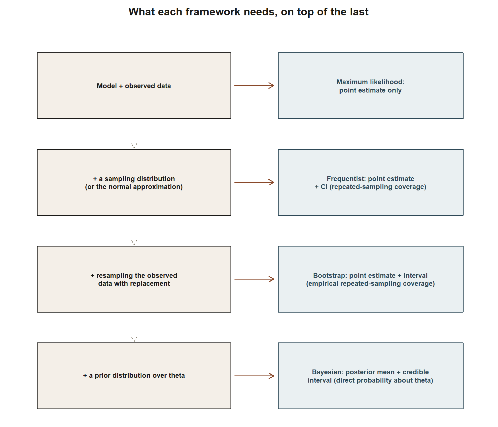
It is also worth naming what raw ingredient each framework needs that the others do not, since that is often the deciding factor in choosing one for a new problem. Maximum likelihood needs only a probability model and the fixed observed data, producing a point estimate rather than an interval in this course’s treatment. The frequentist CI additionally needs a sampling distribution (or a good approximation, like the normal approximation used all term) to attach a long-run coverage guarantee. The bootstrap needs only the observed data and a resampling scheme, trading an analytic formula for computation. The Bayesian posterior needs everything the likelihood needs, plus a prior over the parameter — and in exchange is the only one of the four that licenses a direct probability statement about the parameter itself.

A vertical flow diagram of four rows. Row 1: model plus observed data leads to maximum likelihood, point estimate only. Row 2: plus a sampling distribution or the normal approximation leads to frequentist, point estimate plus confidence interval. Row 3: plus resampling the observed data with replacement leads to bootstrap, point estimate plus interval from empirical repeated-sampling coverage. Row 4: plus a prior distribution over theta leads to Bayesian, posterior mean plus credible interval, a direct probability statement about theta. Dashed arrows connect the left-hand boxes top to bottom, showing each row builds on the last. — Figure 2: **Each framework adds one ingredient to the last (synthetic).** Reading top to bottom, each row’s left-hand box is the previous row’s ingredient plus one new addition; the right-hand box shows what that buys — from a bare point estimate (maximum likelihood) up to a full probability distribution over the parameter (Bayesian).

Worked examples

Worked example — MAC Study: the full four-framework comparison table

This is a synthesis week: the recurring MAC-Study usage-rate thread (Weeks 3, 5–8, 10, 12) is itself the worked example. No separate transfer example is used this week, since the whole point is comparing methods already applied to one running case, not introducing a new one.

Recall every locked number this table draws from, all applied to the question “what is π, the population proportion of students using the MAC in a given week?”

Full survey: n = 100, k = 38, so p̂ = 38/100 = 0.38, with SE(p̂) = √(0.38 × 0.62 / 100) ≈ 0.0485.
Small pilot (Weeks 5–6, by-hand MLE demonstration only): n = 5, k = 2, so π̂ = 2/5 = 0.4.
Frequentist 95% CI (Week 7): 0.38 ± 1.96(0.0485) = 0.38 ± 0.0951 = (0.285, 0.475).
Bayesian prior (Week 12): Beta(a = 3, b = 7), prior mean 0.30. Posterior after the full survey: Beta(3 + 38, 7 + 62) = Beta(41, 69), posterior mean 41/110 ≈ 0.373, posterior SD ≈ 0.0459, normal-approximation 95% credible interval 0.373 ± 1.96(0.0459) ≈ (0.283, 0.463).

Assembled side by side:

Framework	Point estimate	95% interval	Width	Center
MLE (full survey)	0.38	—	—	0.38
MLE (small pilot, Wks 5–6 only)	0.4	—	—	0.4
Frequentist (Wk 7)	0.38	(0.285, 0.475)	0.190	0.380
Bootstrap (Wk 10 method, qualitative)	0.38	similar range to frequentist row	≈ 0.19	≈ 0.38
Bayesian (Wk 12)	0.373	(0.283, 0.463)	0.180	0.373

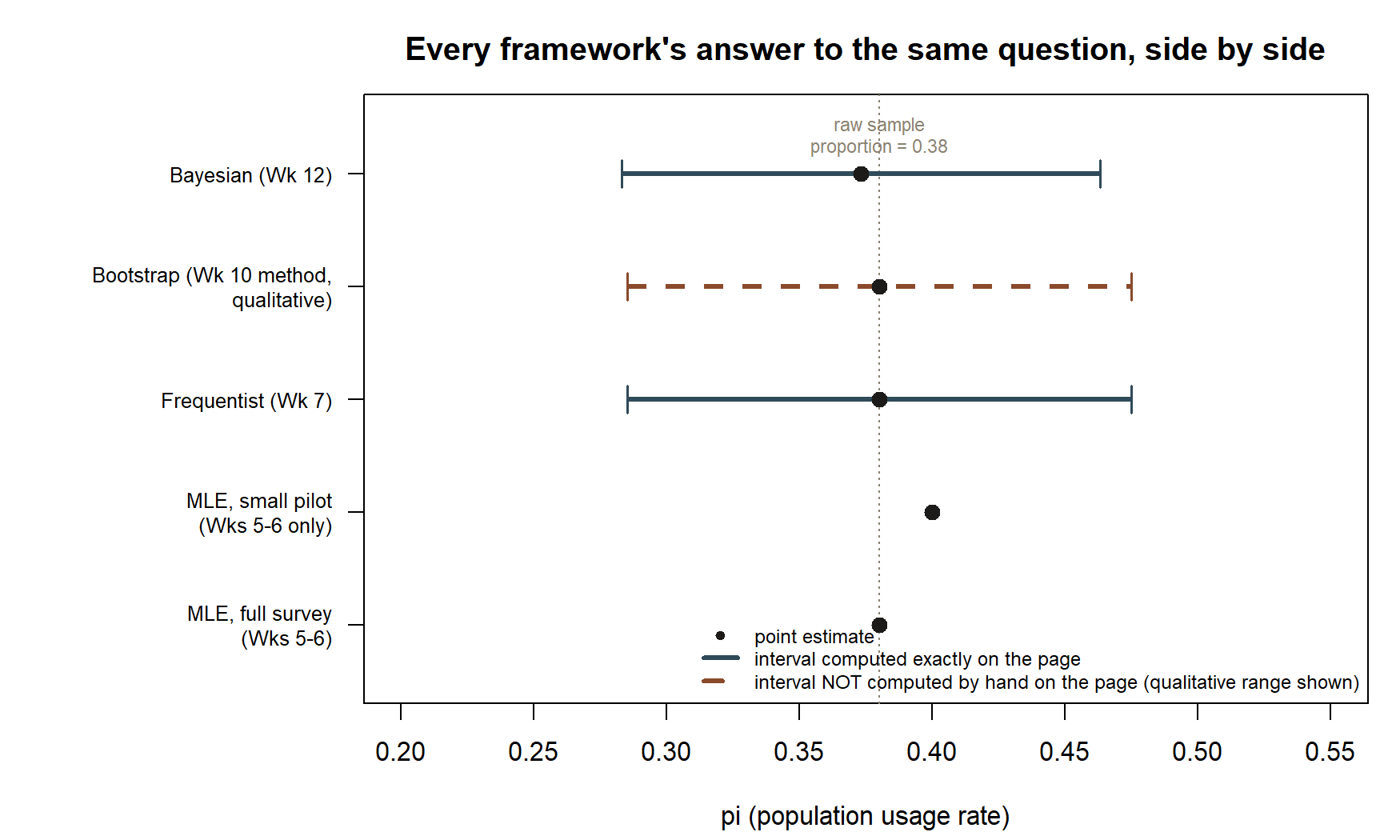
Reading the table: the point estimates cluster tightly (0.373 to 0.4), with the 0.4 pilot value the clear outlier — and that outlier is fully explained by its much smaller sample size (n = 5 vs. n = 100), not by any disagreement about method. The frequentist and Bayesian intervals are close in both center and width, for the reason developed above: a comparatively weak prior (effective sample size 10) updated by a much larger dataset (n = 100) lets the data dominate the posterior. The bootstrap should track the frequentist row closely because the normal approximation is already a good fit to this proportion’s actual sampling distribution. None of this closeness erases the difference in what “95%” means in the frequentist row versus the Bayesian row — that distinction is the point of the “what it claims” column developed in Concept development above, and it does not shrink just because the numbers do.

The table above is easier to scan as a picture — every point estimate and every interval this week has named, lined up on one shared scale:

A dot-and-whisker plot with five rows: Bayesian, bootstrap, frequentist, MLE small pilot, and MLE full survey, all on a pi-axis from 0.20 to 0.55. The Bayesian row shows a dot at 0.373 with a whisker from 0.283 to 0.463. The bootstrap row shows a dot at 0.38 with a dashed whisker from about 0.285 to 0.475, marked qualitative. The frequentist row shows a dot at 0.38 with a whisker from 0.285 to 0.475. The two MLE rows show dots only, at 0.4 and 0.38, with no whiskers. A vertical dotted reference line marks the raw sample proportion 0.38. — Figure 3: **Every framework’s answer, on one scale (synthetic).** Point estimates (dots) and intervals (whiskers) for all five rows of the table above, on the same π-axis. The frequentist and Bayesian whiskers visibly overlap; the pilot MLE sits off to the side, explained by its much smaller sample size rather than by method.

What the figure shows (non-visual equivalent). The Bayesian whisker (0.283, 0.463) and the frequentist whisker (0.285, 0.475) sit almost on top of each other, visually confirming the “where the frameworks agree” discussion above. The bootstrap row is drawn with a dashed whisker matching the frequentist row’s range, because this course does not compute that interval by hand — it is shown as the qualitative range the text argues for, not as an independently computed number. The pilot MLE dot at 0.4 sits apart from the cluster near 0.38, with no whisker at all, since this course’s treatment gives maximum likelihood a point estimate only. Synthetic instructional example; numbers are illustrative.

set.seed(35103)

# Full survey and pilot MLE point estimates
p_hat_full  <- 38 / 100
p_hat_pilot <- 2 / 5

# Frequentist 95% CI for the full survey
se_p <- sqrt(p_hat_full * (1 - p_hat_full) / 100)
ci_freq <- p_hat_full + c(-1, 1) * 1.96 * se_p

# Bayesian posterior (Beta(3,7) prior updated by n=100, k=38)
a_post <- 3 + 38
b_post <- 7 + 62
post_mean <- a_post / (a_post + b_post)
post_var  <- (a_post * b_post) / ((a_post + b_post)^2 * (a_post + b_post + 1))
post_sd   <- sqrt(post_var)
ci_bayes  <- post_mean + c(-1, 1) * 1.96 * post_sd

# Side-by-side summary
data.frame(
  framework = c("MLE (full)", "MLE (pilot)", "Frequentist", "Bayesian"),
  estimate  = c(p_hat_full, p_hat_pilot, p_hat_full, post_mean),
  lower     = c(NA, NA, ci_freq[1], ci_bayes[1]),
  upper     = c(NA, NA, ci_freq[2], ci_bayes[2])
)

A common mistake

Treating “the numbers are close” as evidence that “the frameworks say the same thing.” It is tempting, looking at (0.285, 0.475) and (0.283, 0.463), to conclude that a confidence interval and a credible interval are just two labels for one underlying concept. They are not. The confidence interval is a claim about the long-run behavior of a repeated-sampling procedure; the credible interval is a direct probability statement about the parameter, conditional on a specific prior. These are different logical claims, arrived at by different machinery, that happen to produce similar numbers in this particular case, because this particular prior was weak relative to this particular sample size. Change the prior to something much stronger, or shrink the sample size, and the two intervals can diverge substantially — at which point the “they’re basically the same” intuition breaks down entirely, and only a clear grasp of what each interval actually claims will tell you which one is answering the question you meant to ask.

Low-stakes self-checks (ungraded)

In your own words, write two one-sentence descriptions of what “95%” means — one for the frequentist CI (0.285, 0.475), one for the Bayesian credible interval (0.283, 0.463). Make sure the two sentences are not interchangeable.
The small pilot MLE gave π̂ = 0.4, while the full-survey estimate is p̂ = 0.38. Explain why this difference is about sample size, not about disagreement between methods.
Suppose a colleague had instead used a much stronger prior, Beta(30, 70) (same prior mean 0.30, but ten times the pseudo-observations of the Week 12 prior). Without recomputing exactly, would you expect the resulting posterior mean to sit closer to the prior mean (0.30) or to the sample proportion (0.38), compared to the original Beta(3, 7) posterior mean of 0.373? Why?
Why does this course not carry out a full percentile bootstrap for the usage-rate proportion by hand, and what lets you argue qualitatively that it would land close to the frequentist CI here specifically (rather than needing the argument to hold in general)?
A friend says, “since the CI and the credible interval are almost the same numbers, it doesn’t matter which one you report.” Write two or three sentences explaining what is lost by that claim, using the “what it claims” language from this week.

Reading and source pointer

This week’s synthesis follows MIT OCW 18.05’s review material comparing frequentist and Bayesian approaches to inference, used selectively as this course’s primary spine to frame what each interval formally claims. ModernDive’s treatment of simulation-based inference is the genuinely-used co-source behind this week’s bootstrap discussion — its framing of resampling as an empirical stand-in for a sampling-distribution formula grounds the qualitative bootstrap comparison above, while this course keeps its base-R-only convention rather than ModernDive’s infer-package pipeline. These notes are the course’s own synthesis, grounded in but not copied from the sources.

Public vs. graded

These notes, the examples, and the practice here are public and ungraded — study material only. No graded prompts, answer keys, rubrics, point values, or due dates appear on this site. Graded inference checkpoints, quizzes, homework, labs, the midterm, the project, and the final live in Blackboard (the LMS), which is authoritative for due dates, submissions, and grades. If this page and Blackboard ever disagree, follow Blackboard.

Looking ahead

Week 14 turns this comparison into a decision-making exercise: the inference project workshop asks you to choose at least two of these four frameworks for a new question of your own choosing, and to justify why those two methods (and not the other two) are the right tools for that specific question. Week 15 then pulls the entire term’s MAC-Study thread — every framework, every number, from the Week 1 setup through this week’s comparison — into a single final synthesis picture.