set.seed(35103)

# visit_sample would be the n = 36 recorded visit durations (mean 49.8, SD 15.2).
# One bootstrap resample, drawn with replacement:
one_resample <- sample(visit_sample, size = 36, replace = TRUE)

# Repeat 2000 times, keeping the mean of each resample:
boot_means <- replicate(2000, mean(sample(visit_sample, size = 36, replace = TRUE)))

boot_se <- sd(boot_means)                          # bootstrap SE, ~ 2.53
boot_ci <- quantile(boot_means, c(0.025, 0.975))    # percentile 95% CI, ~ (44.84, 54.76)

hist(boot_means, breaks = 40, freq = FALSE,
     main = "Bootstrap distribution of the mean", xlab = "bootstrap replicate mean (minutes)")
abline(v = 49.8, lty = 1)          # the original sample mean, for comparison
abline(v = boot_ci, lty = 2) # the percentile 95% interval boundariesWeek 10 — Bootstrap inference
Building a confidence interval by resampling the data itself
The week question
Every confidence interval you have built so far — for μ in Week 7, for π in Week 7, for a test statistic in Week 8 — leaned on a formula for the standard error, and that formula leaned on an assumption: a known population SD, or a large enough n for a normal approximation to kick in. This week asks a different question: what if you do not want to assume a specific formula for the standard error, or you are worried that assumption might not hold for a skewed population or a small, unusual sample? Can the data themselves tell you how much a statistic would vary from sample to sample, without your having to derive that variability by formula first?
Why this matters
Real data rarely arrive with a label attached reading “population is exactly Normal” or “σ is known in advance.” The bootstrap is the tool that lets you approximate a statistic’s sampling distribution directly from the one sample you actually have, by treating that sample as a stand-in for the population and resampling from it over and over. It matters for this course in three ways. First, it is a genuinely different strategy from every prior week’s approach: instead of deriving a formula for SE(θ̂) from probability theory, you approximate SE(θ̂) computationally. Second, it generalizes to statistics — a median, a trimmed mean, a correlation, a ratio — where a clean textbook SE formula may not exist or may be hard to derive. Third, it gives you a direct, hands-on check on the formula-based intervals from Week 7: when both approaches apply, does the bootstrap agree with the known-σ interval? Seeing that agreement (or a meaningful disagreement) is itself part of what this week is teaching.
Learning goals
By the end of this week, you should be able to:
- State the bootstrap principle in your own words: resampling with replacement from the observed sample, treating that sample as a working stand-in for the population.
- Explain why the bootstrap does not require a known σ or an assumed normal population.
- Describe how a bootstrap distribution of a statistic is built, step by step, from repeated resamples.
- Compute a bootstrap standard error and a percentile-based bootstrap confidence interval from a set of bootstrap replicate statistics.
- Compare a bootstrap SE and interval against a known-σ, formula-based SE and interval, and explain why they are close but not identical.
- Recognize situations — a skewed quantity, or a statistic without a simple SE formula — where bootstrapping is especially useful.
Core vocabulary
- Bootstrap sample (or resample). A sample of size n drawn with replacement from the original observed sample of size n, so the same original observation can appear zero, one, or several times in a given resample.
- Bootstrap replicate. The value of the statistic of interest (for example, the sample mean) computed on one bootstrap sample.
- Bootstrap distribution. The collection of bootstrap replicates across many resamples (this week, B = 2000 of them), used as an approximation to the statistic’s true sampling distribution.
- Bootstrap standard error. The standard deviation of the bootstrap distribution — an estimate of how much the statistic would vary from sample to sample, built entirely from resampling rather than from a probability formula.
- Percentile bootstrap confidence interval. A confidence interval built directly from percentiles of the bootstrap distribution (or, as shown below, from the bootstrap SE combined with a normal critical value) — no known-σ assumption required.
- Resampling with replacement vs. without replacement. Resampling with replacement is what makes the bootstrap work: it lets each resample differ from the original sample and from every other resample, which is exactly the variability the bootstrap distribution is meant to capture. Resampling without replacement from a fixed sample of size n would just reproduce the same n values in a different order every time — no new variability at all.
Concept development
The problem the bootstrap is solving
Recall the logic behind every confidence interval built so far in this course. To say “θ̂ ± 1.96·SE(θ̂) is a 95% confidence interval,” you need to know how much θ̂ would vary if you repeated the sampling process many times — that is, you need SE(θ̂), the standard deviation of θ̂’s sampling distribution. In Weeks 2, 3, and 7, you got that SE either from a known population SD (a known-σ teaching simplification) or from a large-sample normal approximation formula, such as SE(p̂) = sqrt(p̂(1−p̂)/n). Both routes require either an assumption about the population or a formula that has already been derived for the specific statistic in question.
The bootstrap sidesteps both requirements. Instead of asking “what does probability theory say the sampling distribution of θ̂ looks like,” it asks a more direct, computational question: “if I treat my one observed sample as a stand-in for the population, and I draw many new samples from it — the same way an actual new sample would be drawn from the real population — how much does θ̂ vary across those resamples?” That variability, measured directly from resampling, is used as an approximation to the true sampling variability of θ̂.
The resampling mechanism, step by step
Concretely, given an observed sample of size n:
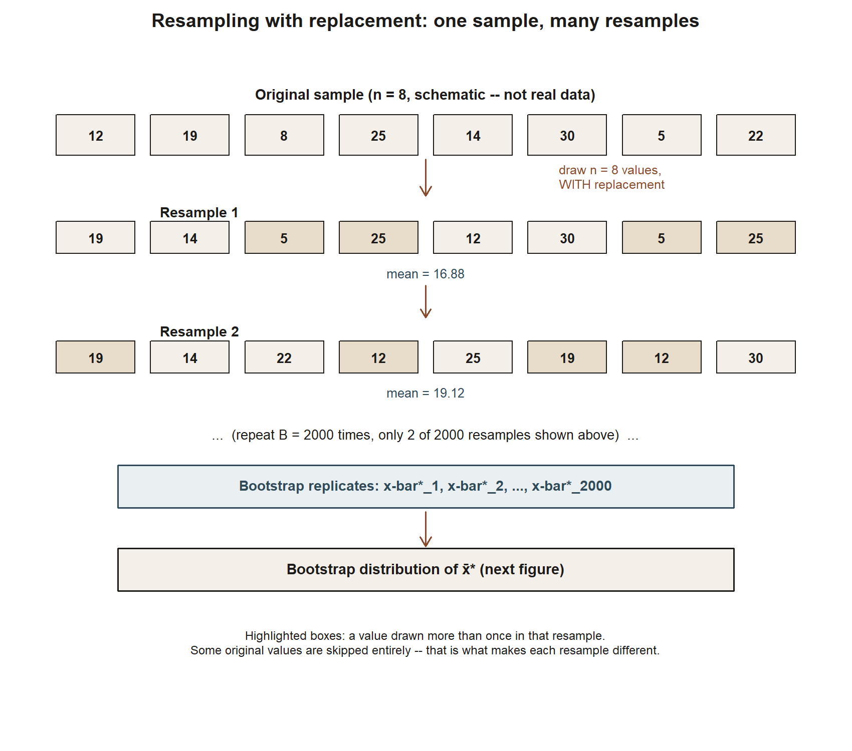
- Draw a resample of size n from the original n observations, with replacement. Because replacement is allowed, a resample is not just a reordering of the original data — some original observations may appear multiple times, and others may not appear at all.
- Compute the statistic of interest (for example, the sample mean) on this resample. This single number is one bootstrap replicate.
- Repeat steps 1 and 2 a large number of times, B (this week’s example uses B = 2000), producing B bootstrap replicates of the statistic.
- Treat the resulting collection of B replicates as an approximation to the statistic’s sampling distribution. Its standard deviation approximates SE(θ̂); its shape and percentiles can be used to build a confidence interval.
Nothing in this mechanism referenced a population σ, a normal-population assumption, or a specific SE formula. The only inputs were the observed sample itself and the resampling process. This is why the bootstrap is described as non-parametric: it does not assume a particular family of distribution for the population.
Seeing the mechanism. The four steps above are easiest to see on a small schematic sample — not the real 36-observation MAC Study data, just a handful of numbers small enough to watch every draw happen.
Why resampling approximates sampling variability
It can feel almost too simple: how can resampling from a sample of size n possibly stand in for drawing a fresh sample of size n from the actual population? The justification is that the observed sample, especially once n is reasonably large, already carries information about the shape of the population — its center, its spread, its skewness. Resampling with replacement from that observed sample generates new “pretend samples” that vary from each other in much the same way repeated real samples from the population would vary, because both kinds of variability trace back to the same underlying spread in the data. The bootstrap distribution is not a perfect stand-in for the true sampling distribution — it is built from one sample, not from repeated access to the population — but under broad conditions it approximates that distribution well enough to be genuinely useful, especially when a clean formula-based SE is unavailable or its assumptions feel shaky.
Worked examples
Worked example — the MAC Study visit-duration bootstrap
Symbolic setup. You have an observed sample of size n with sample mean x̄ and sample SD s. Rather than assuming a known population σ, you resample directly from the observed data:
- Draw B bootstrap resamples of size n, with replacement, from the original n observations.
- Compute the sample mean on each resample, producing bootstrap replicates x̄₁, x̄₂, …, x̄*_B.
- Estimate the bootstrap standard error as the standard deviation of these B replicate means. As a widely used approximation for the mean specifically, this bootstrap SE is close to s/√n, the same form as the known-σ SE formula but built from the sample SD s rather than a population σ.
- Build a percentile-style 95% confidence interval as x̄ ± 1.96 · SE_boot.
Numeric case — the MAC Study. Recall the visit-duration sample from Weeks 2, 3, 7, 8, and 9: n = 36 recorded MAC visits, sample mean x̄ = 49.8 minutes, sample SD s = 15.2 minutes. In Weeks 2 through 9, the population SD was treated as known, σ ≈ 15, giving SE(x̄) = σ/√n = 15/6 = 2.5, and the Week 7 confidence interval for μ was 49.8 ± 1.96(2.5) = 49.8 ± 4.9 = (44.9, 54.7).
This week drops the known-σ assumption. Instead, you resample the 36 visit durations with replacement, B = 2000 times, and compute the mean of each resample. The bootstrap SE approximates s/√n:
\[ SE_{\text{boot}} \approx \frac{s}{\sqrt{n}} = \frac{15.2}{\sqrt{36}} = \frac{15.2}{6} \approx 2.53. \]
Notice this is close to, but not identical to, the known-σ SE of 2.5 from Week 7. That is a deliberate teaching point, not a coincidence to gloss over: the known-σ SE used the hypothetical, stipulated population value σ = 15 (a teaching simplification), while the bootstrap SE is built entirely from the sample SD, s = 15.2, which is itself only an estimate of the unknown true population SD. When the sample SD happens to be close to the value used for the known-σ teaching simplification, the two SEs come out close together — 2.53 versus 2.5 — but they are conceptually different quantities, and only the bootstrap SE would still be available if you refused to assume a known σ at all.
Using the bootstrap SE, the percentile-style 95% confidence interval for μ is:
\[ 49.8 \pm 1.96(2.53) = 49.8 \pm 4.96 \approx (44.84,\ 54.76). \]
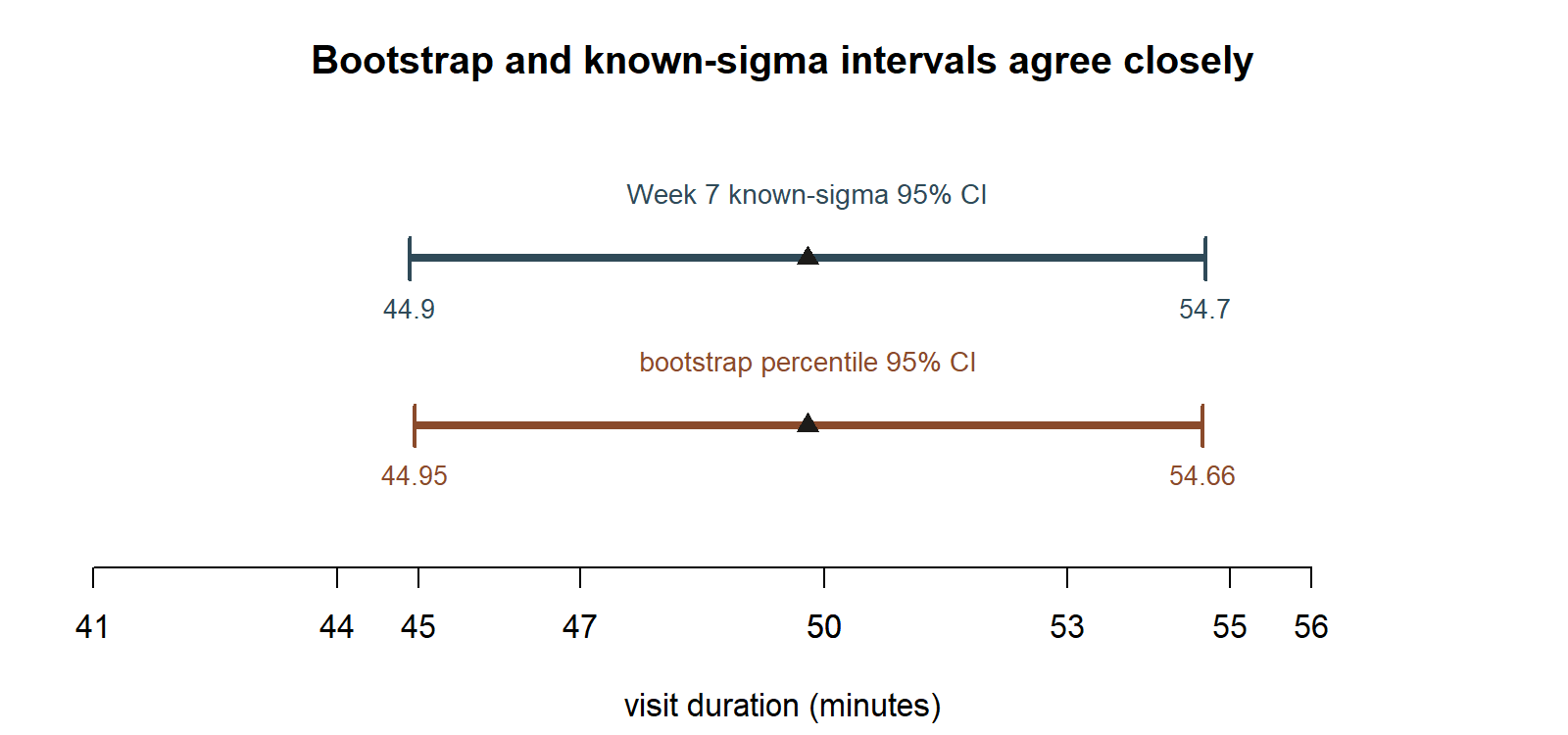
This bootstrap interval, (44.84, 54.76), is extremely close to the Week 7 known-σ interval, (44.9, 54.7) — which is exactly what you should hope to see. The bootstrap did not have access to a known population SD, and yet, by resampling the data 2000 times, it recovered essentially the same interval as the formula that assumed σ was known. That agreement is itself evidence the bootstrap is doing what it claims to do: approximating the same sampling variability the known-σ formula captured analytically, but computationally, directly from the data in hand.
The resampling mechanism in code. The four steps described above translate directly into four lines of base R. (Shown as teaching code, not executed in this build; the companion Lab 10 carries this out in full, step by step, on a synthetic stand-in sample.)
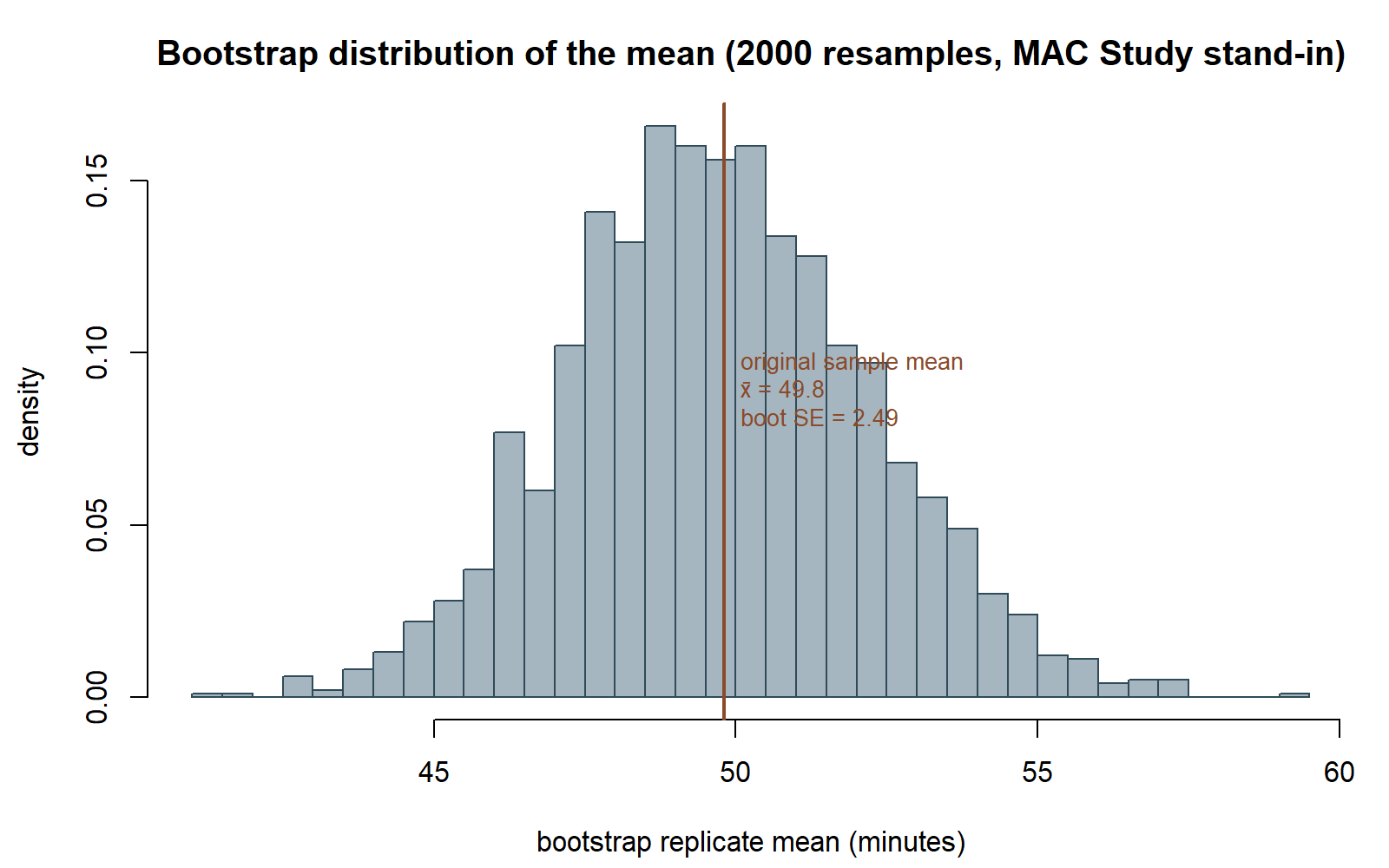
What this shows (public-safe description, since this chunk is not executed here): boot_means becomes a vector of 2000 resample means, its standard deviation approximates the bootstrap SE (\(\approx 2.53\)), and its 2.5th/97.5th percentiles approximate the percentile confidence interval (\(\approx (44.84, 54.76)\)) — the entire bootstrap idea compressed into four lines, with no normal-theory formula anywhere in them.
Seeing the bootstrap distribution. The figure below was produced by running exactly this simulation separately (same seed, set.seed(35103), same n=36, same B=2000), on a synthetic stand-in sample constructed to have exactly the stated mean (49.8) and SD (15.2), so the histogram below is what the chunk above would draw if it were executed.
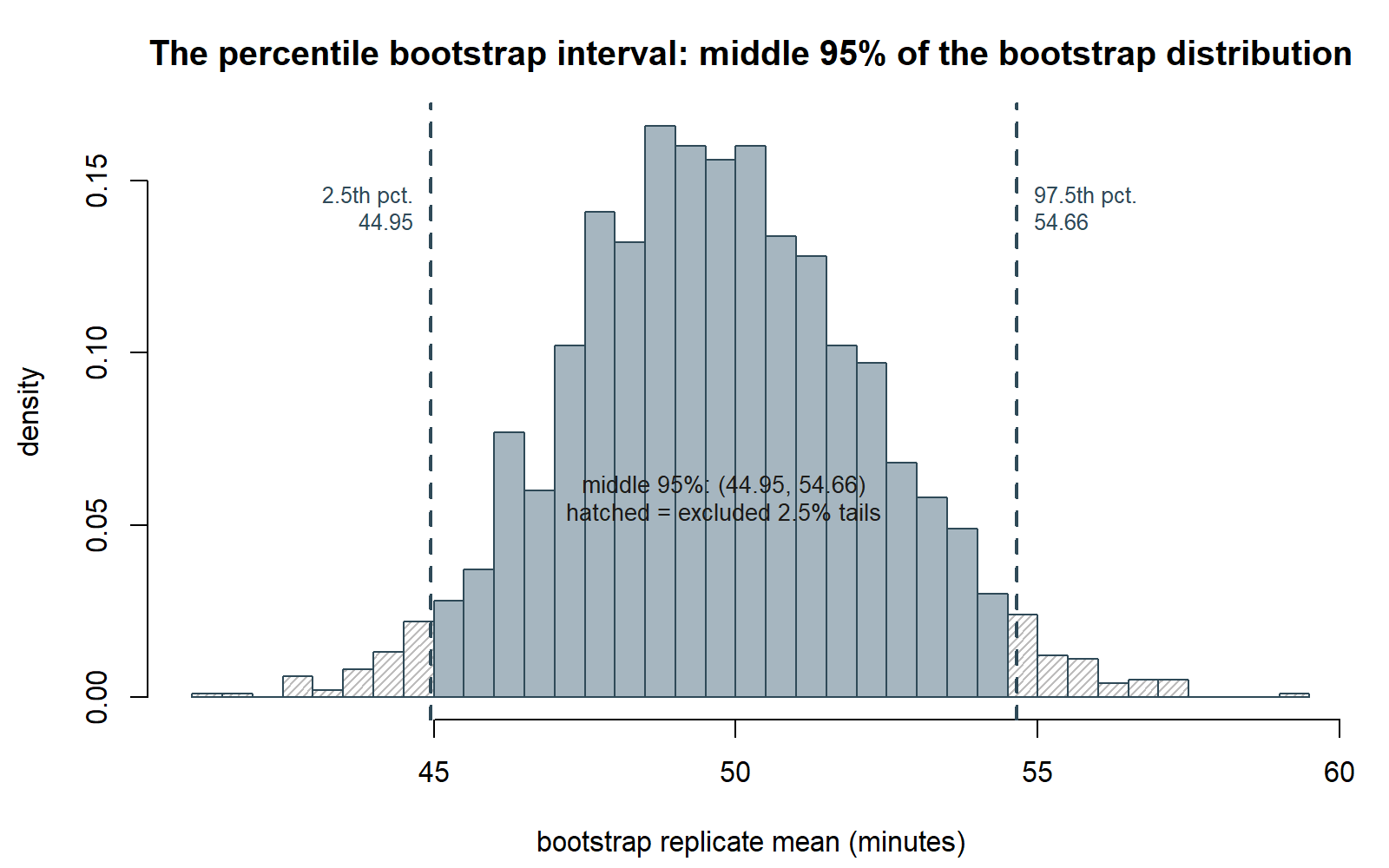
The same histogram is also how you read a confidence interval straight off the data, with no \(\bar{x} \pm 1.96 \cdot SE\) formula at all: cut off the bottom 2.5% and top 2.5% of the 2000 replicates, and whatever remains in the middle is a 95% interval.
Finally, the whole point of this week’s worked example — that the bootstrap recovers essentially the same interval the known-\(\sigma\) formula gave in Week 7 — is easiest to see as two intervals on the same number line.
Worked example — transfer: a bootstrap CI for a skewed household-income median
Symbolic setup. The bootstrap is especially valuable for a statistic like a median, where there is no simple textbook SE formula the way there is for a mean, and where the underlying population may be visibly skewed (income, wait times, and similar quantities are rarely close to normal). The same four-step mechanism applies: resample with replacement from the observed data, compute the median (not the mean) on each resample, collect B replicate medians, and use their spread to build an interval — all without assuming the population of incomes is normally distributed.
Numeric case (synthetic; seed set). Suppose a research team records the household income (in thousands of dollars) for a synthetic sample of n = 40 households in a small survey area, and the sample median income is \(\tilde{x} = 52.0\) thousand dollars. Because income distributions are typically right-skewed (a small number of very high incomes stretch the upper tail), the team does not want to assume normality or rely on a mean-based SE formula. Instead, they bootstrap the median directly:
- Draw B = 2000 resamples of size 40, with replacement, from the 40 observed incomes.
- Compute the median income on each resample, producing 2000 bootstrap replicate medians.
- Suppose (synthetic figures) the standard deviation of these 2000 replicate medians works out to SE_boot ≈ 3.1 thousand dollars, and the 2.5th and 97.5th percentiles of the bootstrap distribution of replicate medians fall at 46.0 and 58.5 thousand dollars.
Reading the interval directly off these percentiles gives a percentile bootstrap 95% confidence interval for the population median income of approximately (46.0, 58.5) thousand dollars — built without ever writing down a formula for the standard error of a median, and without assuming the underlying income distribution is symmetric or normal. This is the case the bootstrap is built for: a statistic (the median) and a population (skewed income) where a normal-theory shortcut either does not exist cleanly or would be a questionable assumption to make.
Seeing the skew. The bullet points above suppose illustrative figures rather than reporting a specific executed run. The figure below runs an actual bootstrap-of-the-median on a genuinely right-skewed synthetic income sample (n=40, seed 35103, B=2000 resamples), so the shape below is a real simulated bootstrap distribution of a median, not a hand-drawn curve.
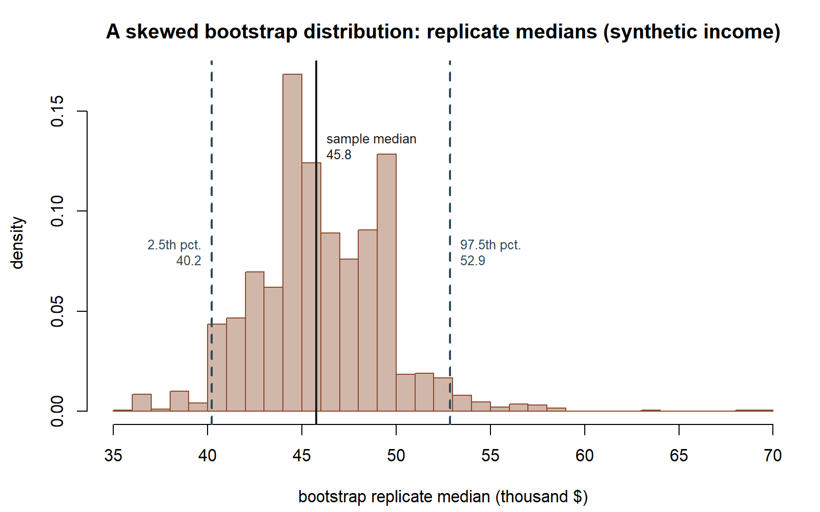
This script’s actual simulated numbers — sample median 45.8, bootstrap SE 3.44, percentile interval (40.22, 52.86) — differ somewhat from the bullet points’ stipulated illustrative figures (median 52.0, SE \(\approx\) 3.1, interval (46.0, 58.5) above), because the two use different synthetic income samples; both are reported here rather than treating one as simply replacing the other. The qualitative lesson is the same either way: the bootstrap distribution of a median from a skewed population is itself not a clean symmetric bell, and the percentile method reads a sensible interval off it regardless.
A common mistake
A common mistake is treating the bootstrap as if it could somehow fix a bad original sample — as though resampling repeatedly from a small or unrepresentative sample could manufacture information about the population that was never in the data to begin with. It cannot. The bootstrap approximates the sampling variability given the observed sample; if that sample is small, biased, or not representative of the population (say, drawn only from one campus building at one time of day), every bootstrap resample inherits the same limitation, and the bootstrap distribution faithfully reproduces that flaw rather than correcting it. The bootstrap approximates sampling variability from a reasonable sample; it is not a substitute for a well-designed sample in the first place.
Low-stakes self-checks (ungraded)
- In your own words, explain why resampling with replacement is essential to the bootstrap, and what would go wrong if you resampled the same n observations without replacement instead.
- Using the MAC Study numbers, explain in a sentence or two why the bootstrap SE (≈2.53) and the known-σ SE (2.5) are close but not identical, referencing where each number comes from.
- Name one statistic other than the mean or median for which you might prefer a bootstrap confidence interval over a normal-theory formula, and say why.
- If a bootstrap distribution of a statistic turned out to be strongly skewed rather than roughly symmetric, would using x̄ ± 1.96·SE_boot (built for a normal-shaped sampling distribution) still be the best way to read a 95% interval from it, or would reading the interval directly off the 2.5th and 97.5th percentiles of the bootstrap distribution make more sense? Explain your reasoning.
Reading and source pointer
This week’s core development follows MIT OCW 18.05’s treatment of bootstrap resampling and simulation-based confidence intervals, which grounds the resampling-with-replacement mechanism and the use of a bootstrap distribution to approximate a sampling distribution. ModernDive’s chapter on bootstrapping is genuinely used alongside 18.05 this week: its framing of building a bootstrap distribution and reading a confidence interval from its percentiles is described here in words and reproduced with base-R resampling (sample() with replace = TRUE, replicate(), and sd()), rather than with ModernDive’s own infer package pipeline. These notes are the course’s own synthesis, grounded in but not copied from the sources.
Public vs. graded
These notes, the examples, and the practice here are public and ungraded — study material only. No graded prompts, answer keys, rubrics, point values, or due dates appear on this site. Graded inference checkpoints, quizzes, homework, labs, the midterm, the project, and the final live in Blackboard (the LMS), which is authoritative for due dates, submissions, and grades. If this page and Blackboard ever disagree, follow Blackboard.
Looking ahead
Next week turns to a different resampling idea: instead of resampling one sample to approximate its own sampling variability, Week 11 reshuffles group labels between two groups to build a null distribution for a group difference from scratch — the randomization (permutation) test. Both weeks share the same spirit of letting the computer, not a textbook formula, generate the distribution you need; Week 11 applies that spirit to a comparison between two groups rather than to a single sample’s statistic.
See also
- Lab 10 — Bootstrap intervals — the companion lab, where you resample the MAC Study visit-duration data yourself in base R and compare the resulting bootstrap interval to the formula-based interval from Week 7.
- Week 7 — Confidence intervals (+ midterm) — the known-σ confidence interval this week’s bootstrap interval is checked against.
- Week 9 — Error rates, power, and decisions — the previous week, where the known-σ framework was used to reason about a testing decision.
- Week 11 — Randomization and permutation tests — next week’s related resampling idea, applied to a two-group comparison.
- Notation glossary — a reference for the symbols used above.