Week 5 — Likelihood

The same data, viewed as a function of the unknown parameter

The week question

You already know how to compute a probability once you’re told a parameter value. If a coin has probability of heads \(\pi = 0.5\), you can compute the probability of any sequence of flips. But an inference problem hands you the opposite situation: you have the data already in hand, and \(\pi\) (or \(\mu\), or whatever parameter governs the process) is the thing you don’t know. This week’s question is: once the data are fixed, how do we use them to say which parameter values are more or less consistent with what we saw? The tool is the likelihood function, \(L(\theta)\), and the discipline of this week is learning to read it correctly — which is harder than it looks, because \(L(\theta)\) looks almost exactly like a probability, and reading it as one is one of the most common errors in a first inference course.

Why this matters

Every estimation method you’ll meet from here forward — maximum likelihood (Week 6), Bayesian updating (Week 12), and even some of the reasoning behind confidence intervals (Week 7) — leans on the likelihood function as the bridge between “the model” and “the data.” Before you can maximize a likelihood, compare two likelihoods, or turn a likelihood into a posterior, you need a very precise sense of what \(L(\theta)\) is and is not. Get the direction of the function backwards — treat it as a probability distribution over \(\theta\) instead of a function of \(\theta\) for fixed data — and every formula you write down afterward will be formally fine but conceptually broken. This week exists to build that precision before Week 6 asks you to maximize it.

Learning goals

By the end of this week you should be able to:

• State, in your own words, the difference between a probability (function of data, parameter fixed) and a likelihood (function of the parameter, data fixed).
• Write down the likelihood function for a Binomial setting, \(L(\pi) \propto \pi^{k}(1-\pi)^{n-k}\), given observed data \(n\) and \(k\).
• Evaluate \(L(\theta)\) at several candidate values of \(\theta\) and compare them to say which value the data favor more.
• Explain why \(L(\theta)\) does not need to integrate to 1 over \(\theta\), and why that matters for what you’re allowed to conclude from it.
• Name the common mistake of reading \(L(\theta)\) as “the probability that \(\theta\) is true” and say why it’s wrong.

Core vocabulary

• Likelihood function, \(L(\theta)\). A function of the parameter \(\theta\), built from data that are already fixed/observed. For a Binomial count of \(k\) successes in \(n\) trials, \(L(\pi) = \binom{n}{k} \pi^{k}(1-\pi)^{n-k}\), or, dropping the constant \(\binom{n}{k}\) that doesn’t depend on \(\pi\), the likelihood kernel \(\pi^{k}(1-\pi)^{n-k}\).
• Probability (for contrast). A function of the data (or of an event), for a fixed parameter value. “If \(\pi = 0.4\), the probability of seeing exactly \(k=2\) successes in \(n=5\) trials” is a probability statement — \(\pi\) is fixed, the data are what varies.
• Likelihood kernel. The part of the likelihood that depends on \(\theta\); constants that don’t involve \(\theta\) (like \(\binom{n}{k}\) above) can be dropped because they don’t affect which \(\theta\) the data favor most — they scale every value of \(L(\theta)\) by the same amount.
• Log-likelihood, \(\ell(\theta) = \ln L(\theta)\). The natural log of the likelihood. Not derived in detail until Week 6, but worth having the name now: taking logs turns products into sums, which is why it shows up as soon as you start maximizing.
• Relative likelihood / likelihood comparison. Comparing \(L(\theta_1)\) to \(L(\theta_2)\) for the same fixed data tells you which of the two parameter values the data support more strongly — a comparison, not an absolute probability statement about either value.

Concept development

Two functions that look alike but point in opposite directions

Start from the same underlying model in both directions. Suppose a single coin flip (or a single MAC-usage check, or any binary outcome) succeeds with probability \(\pi\). If you fix \(\pi\), you can ask: “what’s the probability of this or that data outcome?” That’s an ordinary probability question, and \(\pi\) is a known constant while the data outcome is what’s uncertain.

Now flip the roles. Suppose you’ve already run the study — the data are sitting in front of you, unchanging — and \(\pi\) is what you don’t know. You can still write down the exact same mathematical expression, \(\pi^{k}(1-\pi)^{n-k}\), but now you’re going to walk it as a function of \(\pi\), holding \(k\) and \(n\) fixed at their observed values. That walked-as-a-function-of-\(\pi\) object is the likelihood function, \(L(\pi)\).

Symbolically, for a Binomial count of \(k\) successes in \(n\) independent trials with success probability \(\pi\):

\[P(K = k \mid \pi) = \binom{n}{k}\pi^{k}(1-\pi)^{n-k}, \qquad k \text{ varies}, \ \pi \text{ fixed (probability)}\]

\[L(\pi) = \binom{n}{k}\pi^{k}(1-\pi)^{n-k}, \qquad \pi \text{ varies}, \ k \text{ (and } n\text{) fixed (likelihood)}\]

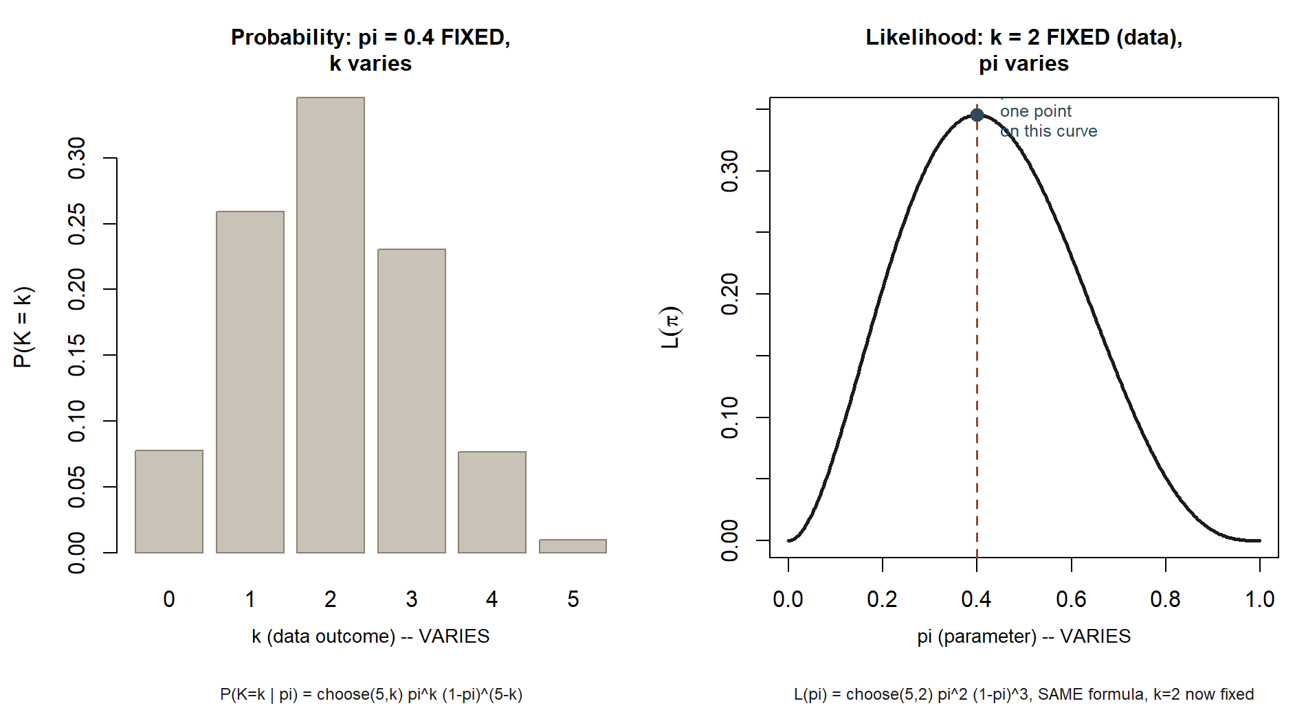
The formula on the page is identical. What changed is which symbol you’re allowed to move. This is the single idea the rest of the week builds on, and it is worth re-reading until it feels obvious, because almost every downstream mistake in likelihood-based reasoning traces back to forgetting which side of this contrast you’re standing on.

Seeing the contrast directly. The same \(n=5\) setup, drawn as two pictures side by side, makes the “which symbol moves” question impossible to miss:

Figure 1: Same formula, opposite direction (synthetic). Left: probability, with \(\pi=0.4\) held fixed and the data outcome \(k\) ranging over every possible value \(0,\dots,5\) — a bar chart that sums to 1. Right: likelihood, with the observed \(k=2\) held fixed and the parameter \(\pi\) ranging continuously over \((0,1)\) — a curve that does not sum or integrate to 1.

What the figure shows (non-visual equivalent). Both panels use the exact same formula, \(\binom{5}{k}\pi^{k}(1-\pi)^{5-k}\). The left panel fixes \(\pi=0.4\) and varies \(k\) across its six possible values — a genuine probability distribution, bars summing to 1. The right panel fixes the observed \(k=2\) and varies \(\pi\) continuously — the likelihood function, a curve that does not sum or integrate to 1 (see the figure later in this section that shows this directly). The value \(\pi=0.4\) that is one bar’s condition on the left becomes one point on a continuous curve on the right — same number, two entirely different roles. Synthetic instructional example; numbers are illustrative.

Why \(L(\theta)\) is not a probability distribution over \(\theta\)

A probability distribution over a parameter \(\theta\) would need to satisfy the basic rules of probability: non-negative values, and — for a continuous parameter — total area 1 when integrated over all possible \(\theta\). \(L(\theta)\) satisfies the first (it can’t be negative, since it’s built from probabilities or densities), but not the second. If you integrated \(L(\pi) = \pi^{k}(1-\pi)^{n-k}\) over \(\pi\) from 0 to 1, you would not, in general, get 1. There is no rule that forces it to.

Figure 2: The area under a likelihood curve is not 1 (synthetic). The same MAC-Study pilot likelihood kernel \(L(\pi)=\pi^2(1-\pi)^3\) from below, with the area under its own curve from \(\pi=0\) to \(\pi=1\) shaded and numerically integrated: the total is about \(0.0167\), not 1.

What the figure shows (non-visual equivalent). The shaded region is the entire area under the MAC-Study pilot’s likelihood kernel \(L(\pi)=\pi^2(1-\pi)^3\), integrated over every possible \(\pi\) from 0 to 1. That area comes out to about \(0.0167\) — nowhere near 1. A genuine probability density over \(\pi\) would have to integrate to exactly 1; this curve does not, which is the concrete reason \(L(\pi)\) cannot be read as “the probability distribution of \(\pi\).” Synthetic instructional example; numbers are illustrative.

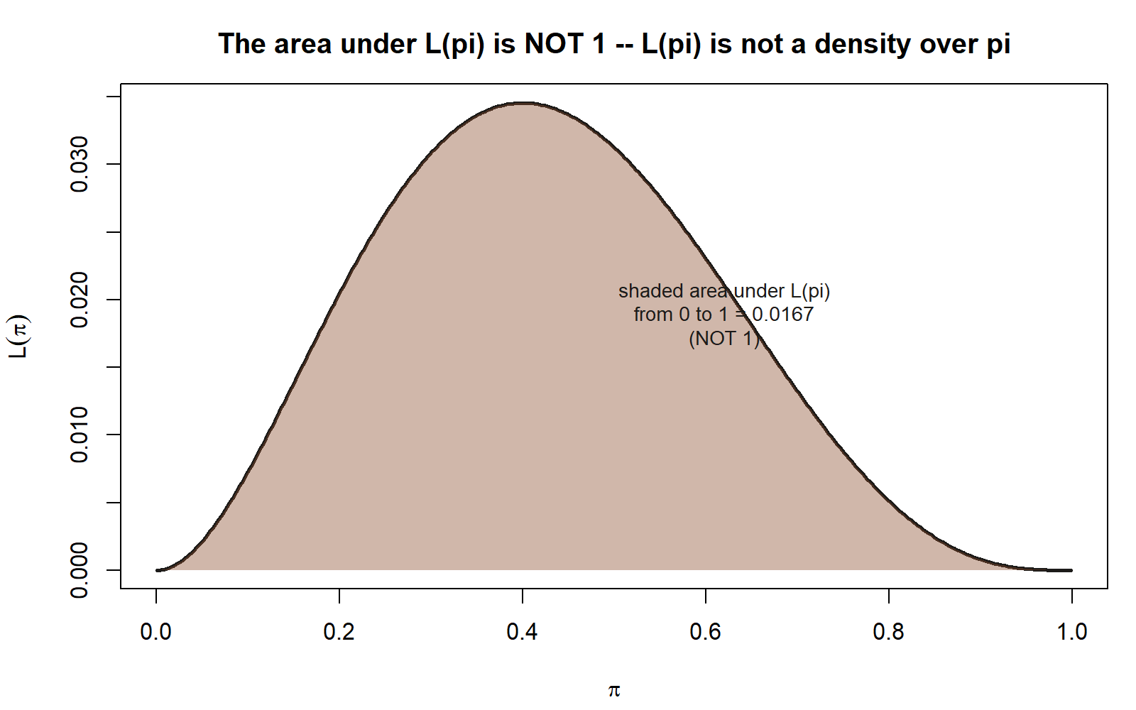
This matters practically: you cannot ask “what fraction of the total likelihood sits between \(\pi = 0.3\) and \(\pi = 0.5\)?” and interpret the answer as a probability that \(\pi\) is in that range. The likelihood function supports relative statements — “\(\theta_1\) is more consistent with the data than \(\theta_2\),” or later, “this is the single most likely value of \(\theta\) given the data” — but not the absolute probability statements that a genuine distribution over \(\theta\) would support. Building that kind of absolute statement about \(\theta\) requires a prior distribution and Bayes’ rule, which is exactly the machinery Week 12 introduces. Until then, keep \(L(\theta)\) and any future \(\pi(\theta \mid \text{data})\) (the Bayesian posterior) visually and verbally distinct — this course flags that boundary every time it’s relevant, and this is the first time it bites.

Reading a likelihood function as a comparison tool

Because \(L(\theta)\) isn’t a probability distribution, the natural use of it isn’t to read off a single number and interpret it in isolation — a lone value like \(L(0.4) = 0.03456\) has no meaning by itself; it depends on units, sample size, and how the kernel was scaled. The natural use is comparison: evaluate \(L(\theta)\) at two or more candidate values of \(\theta\), using the same fixed data both times, and see which one is larger. A larger \(L(\theta_1)\) than \(L(\theta_2)\) means the observed data are more consistent with \(\theta_1\) than with \(\theta_2\) — nothing more, nothing less, but that “more consistent with” comparison is exactly the seed that Week 6 grows into a full estimation method: search over all possible \(\theta\) and find the one that makes \(L(\theta)\) largest. This week stops one step short of that maximization — the goal here is only to get comfortable computing and comparing \(L(\theta)\) at a few candidate values, not yet to find the single best one.

Worked examples

Worked example — the MAC Study: a small pilot batch

Before the full \(n=100\) MAC-usage survey (Week 3’s thread) was collected, the research team ran a small pilot: the first five survey responses came in, and \(k = 2\) of the five students said they’d used the MAC at least once that week. This pilot batch is deliberately small and separate from the full survey — kept small on purpose so the likelihood arithmetic is tractable by hand.

Let \(\pi\) denote the (unknown) population proportion of students who use the MAC in a given week. With \(n=5\) trials and \(k=2\) observed successes, the likelihood kernel is:

\[L(\pi) \propto \pi^{k}(1-\pi)^{n-k} = \pi^{2}(1-\pi)^{3}\]

(The kernel drops the binomial coefficient \(\binom{5}{2}=10\), since it’s a constant that doesn’t depend on \(\pi\) and doesn’t change which \(\pi\) the data favor most — it would just scale every evaluation below by the same factor of 10.)

Now evaluate the kernel at three candidate values of \(\pi\), treating \(k=2\) and \(n=5\) as fixed throughout:

\[L(0.2) = (0.2)^2(0.8)^3 = (0.04)(0.512) = 0.02048\]

\[L(0.4) = (0.4)^2(0.6)^3 = (0.16)(0.216) = 0.03456\]

\[L(0.6) = (0.6)^2(0.4)^3 = (0.36)(0.064) = 0.02304\]

Lay the three side by side: \(L(0.2) = 0.02048\), \(L(0.4) = 0.03456\), \(L(0.6) = 0.02304\). Among these three candidate values, \(\pi = 0.4\) has the largest likelihood — the observed pilot data (\(k=2\) out of \(n=5\), a sample proportion of \(\hat\pi = 2/5 = 0.4\)) are more consistent with \(\pi = 0.4\) than with either \(\pi = 0.2\) or \(\pi = 0.6\). Notice that \(0.4\) is also just the sample proportion \(k/n\) — that is not a coincidence, and Week 6 will show exactly why the sample proportion is the value that maximizes this likelihood over every possible \(\pi\) in \([0,1]\), not just the three candidates checked here.

set.seed(35103)

# Small illustrative pilot batch: n = 5, k = 2 used the MAC.
n <- 5
k <- 2

likelihood_kernel <- function(pi) {
  pi^k * (1 - pi)^(n - k)
}

candidates <- c(0.2, 0.4, 0.6)
sapply(candidates, likelihood_kernel)
# Compare to the sample proportion k/n = 0.4 — foreshadowing next week's MLE.

Three isolated numbers only go so far. The shape of \(L(\pi)\) across every candidate value, not just the three checked above, is what a likelihood curve shows directly — and it is the canonical picture for this week’s idea, so it is worth building explicitly rather than only imagining it.

Figure — the MAC-Study pilot likelihood curve. The code below evaluates the same kernel over a fine grid of \(\pi\) values from 0 to 1 and plots the resulting curve. Shown as teaching code, not executed in this build (eval: false) — running it yourself is the point, and predicting its shape before you look is a useful check on your own understanding.

set.seed(35103)

# Same n = 5, k = 2 pilot batch as above, now evaluated over a fine grid of pi.
n <- 5
k <- 2
pi_grid <- seq(0.01, 0.99, by = 0.01)

likelihood_curve <- dbinom(k, size = n, prob = pi_grid)   # proportional to the kernel above

plot(pi_grid, likelihood_curve, type = "l",
     xlab = expression(pi), ylab = expression(L(pi)),
     main = "Likelihood curve: MAC-Study pilot (n = 5, k = 2)")
abline(v = k / n, lty = 2)   # marks the peak at pi = 0.4, foreshadowing Week 6's MLE

The figure below was produced by running exactly this computation separately (same \(n=5\), \(k=2\), same fine grid of \(\pi\)), so you can check your own prediction against a real result:

Figure 3: The MAC-Study pilot likelihood curve (synthetic). \(L(\pi)=\pi^2(1-\pi)^3\) over the full range \(\pi \in (0,1)\), peaking at \(\pi=0.4\). The three points already computed by hand above — \(L(0.2)=0.02048\), \(L(0.4)=0.03456\), \(L(0.6)=0.02304\) — sit exactly on this curve, on the rising side, at the peak, and on the falling side, respectively.

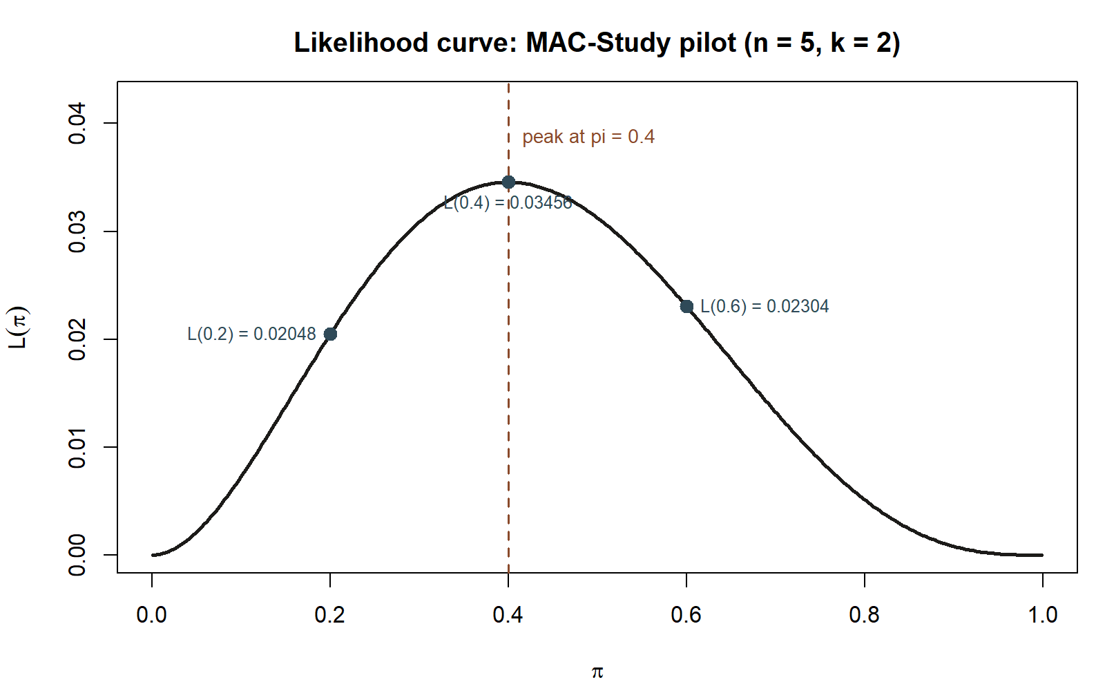
What this shows: the three isolated numbers computed by hand above are all points on one continuous curve, and that curve makes visually obvious what the three numbers only suggested — \(\pi=0.4\) is not just the tallest of three candidates, it is the single highest point anywhere on the curve (Week 6 makes that “single highest point” claim exact, by calculus, instead of by eye). Synthetic instructional example; numbers are illustrative.

Worked example — transfer: is this coin fair?

Synthetic; seed set. Move to a fresh, unrelated context to check the idea transfers: assessing whether a coin is fair from a small number of flips. Suppose you flip a coin \(n=4\) times (synthetic data, not part of the MAC Study) and observe \(k=3\) heads. Let \(\pi\) denote the true probability of heads for this particular coin. The likelihood kernel, exactly parallel to the MAC-Study case, is:

\[L(\pi) \propto \pi^{k}(1-\pi)^{n-k} = \pi^{3}(1-\pi)^{1}\]

Compare two candidate values: a “fair coin” hypothesis, \(\pi = 0.5\), against the sample proportion, \(\pi = 3/4 = 0.75\):

\[L(0.5) = (0.5)^3(0.5)^1 = (0.125)(0.5) = 0.0625\]

\[L(0.75) = (0.75)^3(0.25)^1 = (0.421875)(0.25) = 0.10546875\]

\(L(0.75) \approx 0.1055\) is noticeably larger than \(L(0.5) = 0.0625\) — this small, synthetic sample of four flips is more consistent with \(\pi = 0.75\) than with the fair-coin value \(\pi = 0.5\). That does not mean you should conclude the coin is unfair; with only \(n=4\) flips, the likelihood function is quite flat, and a value near 0.5 is still plausible. What the comparison licenses is a narrower claim: among the two candidate values checked, the data lean toward \(\pi = 0.75\) over \(\pi = 0.5\). Whether that lean is strong enough to act on is a question for later weeks (hypothesis testing, Week 8; confidence intervals, Week 7) — this week’s job is only to compute and compare \(L(\theta)\) correctly, not yet to decide how much evidence is “enough.”

Figure 4: The transfer coin-example likelihood curve (synthetic). \(L(\pi)=\pi^3(1-\pi)^1\) over \(\pi \in (0,1)\) for the \(n=4\), \(k=3\) coin flips, peaking at the sample proportion \(\pi=0.75\). The two compared candidates, \(L(0.5)=0.0625\) and \(L(0.75)\approx0.1055\), sit on the curve as marked points — \(\pi=0.75\) is higher, but the curve is visibly flat and wide with only \(n=4\) flips.

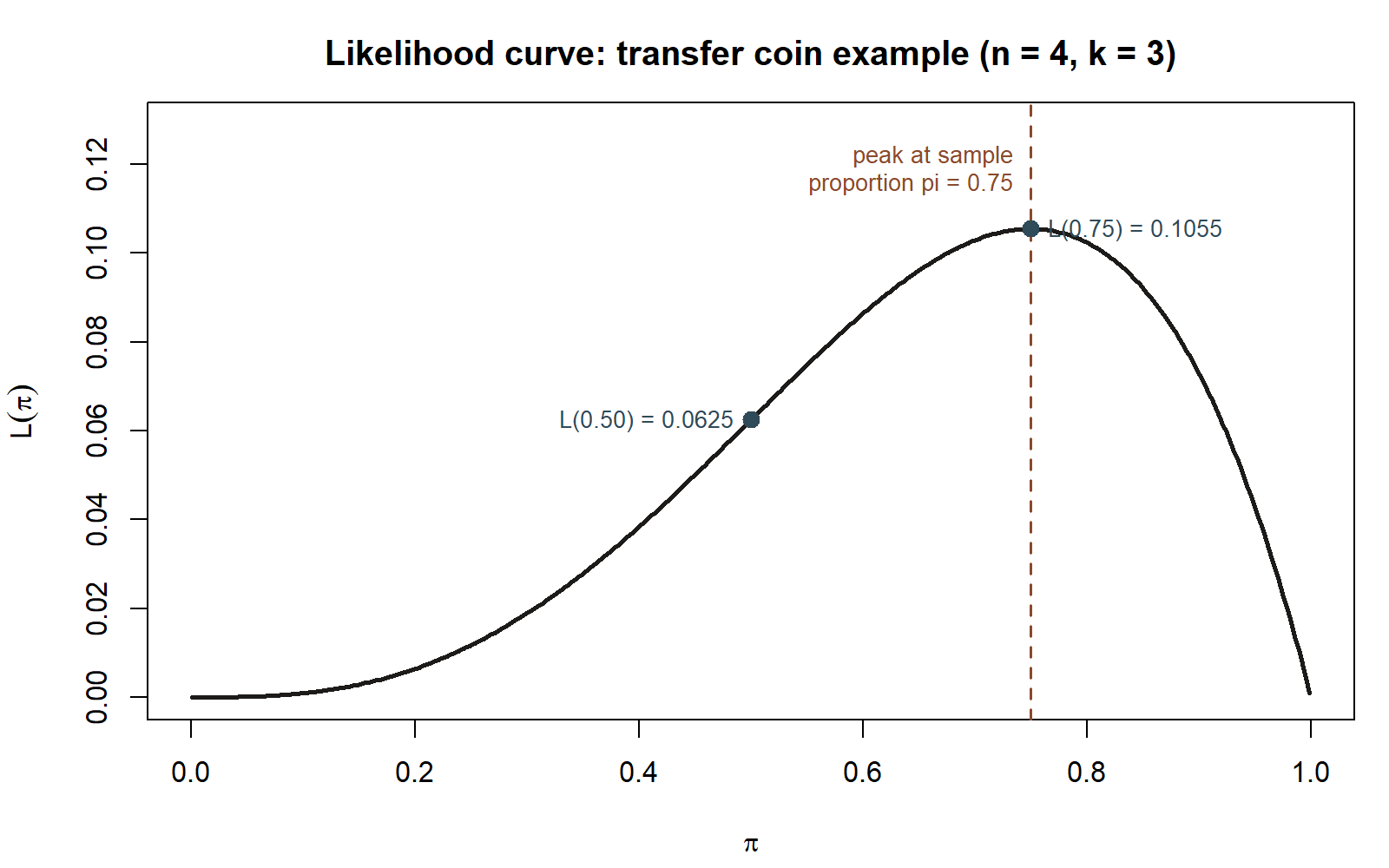
What this shows: the curve makes the “flat and wide” warning in the paragraph above literal — with only four flips, the likelihood does not fall off sharply away from its peak, so several values of \(\pi\) besides \(0.75\) still have a reasonably large likelihood. Synthetic instructional example; numbers are illustrative.

set.seed(35103)

# Synthetic transfer example: n = 4 flips, k = 3 heads.
n <- 4
k <- 3

likelihood_kernel <- function(pi) {
  pi^k * (1 - pi)^(n - k)
}

candidates <- c(0.5, 0.75)
sapply(candidates, likelihood_kernel)

A common mistake

The single most common error at this stage is reading \(L(\theta)\) as if it were a probability distribution over \(\theta\) — for instance, saying “\(L(0.4) = 0.03456\) means there’s a 3.456% chance that \(\pi = 0.4\).” This is wrong on two counts. First, \(L(\theta)\) generally does not integrate (or sum, for a discrete parameter grid) to 1 across all possible \(\theta\), so its raw values are not probabilities in the ordinary sense — they don’t even have a fixed scale, since dropping or keeping a multiplicative constant like \(\binom{n}{k}\) changes every value without changing anything you’re entitled to conclude. Second, and more fundamentally, making a genuine probability statement about \(\theta\) requires a prior distribution over \(\theta\) and Bayes’ rule to combine it with the data — that’s the posterior distribution \(\pi(\theta \mid \text{data})\), introduced formally in Week 12, not the likelihood alone. Until then, the only sound reading of \(L(\theta)\) is relative: it tells you which candidate values of \(\theta\) are more or less consistent with the data you already have, not how probable any one of them is.

Low-stakes self-checks (ungraded)

• In your own words, explain the difference between “the probability of the data given \(\theta\)” and “the likelihood of \(\theta\) given the data.” What symbol is fixed in each, and what symbol varies?
• Using the MAC-Study pilot (\(n=5\), \(k=2\)), evaluate the likelihood kernel \(\pi^2(1-\pi)^3\) at \(\pi = 0.3\) and at \(\pi = 0.5\). Which of the two is more consistent with the pilot data? (Compare each to the three values already worked above: \(L(0.2)=0.02048\), \(L(0.4)=0.03456\), \(L(0.6)=0.02304\).)
• For the transfer coin example (\(n=4\), \(k=3\)), evaluate \(L(0.9)\) and compare it to \(L(0.75) \approx 0.1055\) computed above. Does the data favor \(\pi = 0.9\) or \(\pi = 0.75\) more?
• Why can’t you say “the area under \(L(\theta)\) between \(\pi=0.3\) and \(\pi=0.5\) gives the probability that \(\pi\) is in that range”? Name the missing ingredient that would let you make a genuine probability statement about \(\theta\).
• A classmate says, “the likelihood function shows all the probable values of \(\pi\), weighted by how likely each one is.” Identify exactly what’s wrong with that sentence, using this week’s vocabulary.

Reading and source pointer

This week’s development of the likelihood function follows MIT OCW 18.05’s treatment of likelihood, used selectively as this course’s primary spine — its framing of the likelihood function as a function of the parameter for fixed data, and the probability-vs-likelihood contrast, both ground this week’s presentation. These notes are the course’s own synthesis, grounded in but not copied from the sources.

Public vs. graded

These notes, the examples, and the practice here are public and ungraded — study material only. No graded prompts, answer keys, rubrics, point values, or due dates appear on this site. Graded inference checkpoints, quizzes, homework, labs, the midterm, the project, and the final live in Blackboard (the LMS), which is authoritative for due dates, submissions, and grades. If this page and Blackboard ever disagree, follow Blackboard.

Looking ahead

Week 6 picks up exactly where this week stops: instead of comparing \(L(\theta)\) at a handful of candidate values, you’ll maximize it over every possible value of \(\theta\), deriving the maximum likelihood estimate \(\hat\theta_{\text{MLE}}\) symbolically for both the Binomial proportion and the Normal mean. The same MAC-Study pilot batches — the \(n=5, k=2\) usage pilot and a companion small sample of five visit durations — carry straight over, so the numbers you computed this week become the launching point for that derivation.

See also

• Week 4 — Bias, variance, and mean squared error
• Week 6 — Maximum likelihood estimation
• Notation glossary
• Inference formula reference