set.seed(35103)

# Mean CI: MAC visit duration (known-sigma teaching simplification)
xbar <- 49.8
se_mean <- 15 / sqrt(36)
ci_mean <- xbar + c(-1, 1) * 1.96 * se_mean
ci_mean

# Proportion CI: MAC usage rate
phat <- 0.38
se_prop <- sqrt(phat * (1 - phat) / 100)
ci_prop <- phat + c(-1, 1) * 1.96 * se_prop
ci_propWeek 7 — Confidence intervals (+ midterm)
Turning a point estimate and a standard error into an honest range
A scheduling note before anything else: the midterm is Friday, Oct 9, in class, and covers first-half material — sampling distributions through confidence intervals. Nothing on this page is graded. This note is study material only; the midterm itself, its coverage details, and any review guide Blackboard posts are handled there, not here (see Public vs. graded below).
The week question
You have a point estimate — a single number like x̄ = 49.8 or p̂ = 0.38 — and a standard error that tells you roughly how much that number would jiggle from sample to sample. How do you turn those two ingredients into a range of plausible values for the unknown parameter, and — the harder question — what does that range actually mean once you have it?
Why this matters
A point estimate alone hides its own uncertainty. Reporting “the average MAC visit lasts 49.8 minutes” sounds precise, but it is a single draw from a noisy process; a different week’s sample of the same size would almost certainly produce a different x̄. A confidence interval reports the estimate and a calibrated sense of how far off it might be, using exactly the standard error machinery built in Week 3. Confidence intervals are also the natural bridge into Week 8’s hypothesis tests: both use the same standardized distance between an estimate and a reference value, just aimed at different questions (“what’s plausible?” vs. “is this specific value rejectable?”).
Learning goals
By the end of this week you should be able to:
- State the general form of a confidence interval: estimate ± (critical value) × SE(estimate).
- Construct a 95% CI for a population mean μ (known σ case) and for a population proportion π, using the sample facts already in hand from the MAC Study.
- Explain, in words a non-statistician would accept, what “95% confidence” actually describes — a property of the repeated-sampling procedure, not a probability statement about one specific interval.
- Name and avoid the single most common CI misinterpretation.
- Recognize how interval width depends on confidence level, standard error, and sample size.
Core vocabulary
- Confidence interval (CI): a range of values, computed from sample data, constructed so that the procedure used to build it captures the true parameter a specified percentage of the time over repeated sampling. A CI is a property of the procedure — never a probability statement about a single realized interval.
- Confidence level: the long-run success rate of the procedure (e.g., 95%), chosen in advance, not a property discovered after seeing the data.
- Critical value: the multiplier attached to the standard error, drawn from the reference distribution (for a 95% CI under normal theory, 1.96 from the standard normal).
- Margin of error: the “plus-or-minus” piece of the interval — critical value times SE(estimate).
- Coverage: the actual long-run proportion of intervals (built the same way, over hypothetical repeated samples) that contain the true parameter; for a correctly derived 95% procedure, coverage is 0.95.
Concept development
The general recipe
Every confidence interval in this course has the same skeleton:
\[ \text{estimate} \;\pm\; (\text{critical value}) \times SE(\text{estimate}). \]
The “estimate” is whatever point estimator you are using (x̄ for μ, p̂ for π). The “critical value” comes from the sampling distribution of that estimator — under the normal approximations used through Week 9, a 95% CI uses z* = 1.96, the value that leaves 2.5% of the standard normal distribution in each tail. The SE is exactly the standard error built in Week 3: SE(x̄) = σ/√n for a mean (known σ), SE(p̂) = √(p̂(1−p̂)/n) for a proportion.
Widening the confidence level (say, to 99%) increases the critical value (to about 2.576), which widens the interval — you buy more confidence by admitting a wider range of plausible values. Increasing n shrinks the SE, which narrows the interval for the same confidence level — more data buys precision without giving up confidence. These two levers (confidence level and sample size) are the only way to trade off width against reliability; there is no way to get a narrower interval at the same confidence level without more data (or a less variable population).
Why 1.96, and what “95%” is really describing
Under the normal approximation, a standardized estimate — like \((\bar{x}-\mu)/SE(\bar{x})\) — behaves like a standard normal variable across repeated samples. Exactly 95% of standard normal draws fall between −1.96 and +1.96. So if you always build the interval x̄ ± 1.96·SE(x̄), then in 95% of hypothetical repeated samples the resulting interval will straddle the true (unknown) μ — because in 95% of samples, x̄ itself will have landed within 1.96 standard errors of μ.
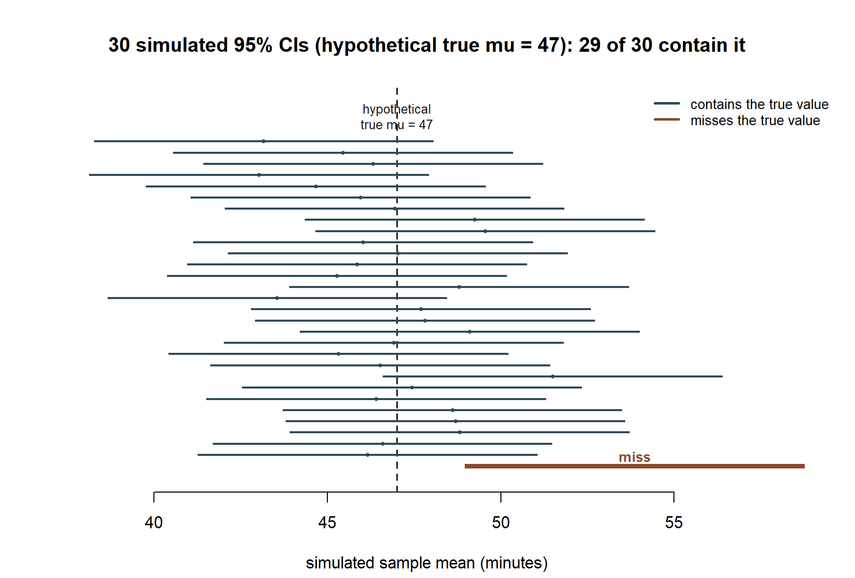
This is the crucial shift in perspective: before you draw the sample, the interval’s endpoints are random (they depend on whatever x̄ you happen to get), while μ is fixed. The randomness lives entirely in the sampling procedure, not in the parameter. Once you actually draw one sample and compute one specific interval, like (44.9, 54.7), that interval either does or does not contain the true μ — there is no more randomness left to attach a 95% probability to. The 95% describes the track record of the method, evaluated across all the samples you didn’t happen to draw.
Seeing “95%” as a track record, not a single-interval probability. The figure below simulates exactly that repeated-sampling story: 30 hypothetical samples (n = 36, SE = 2.5), each producing its own 95% CI, built around a stipulated hypothetical true value μ = 47 (chosen only so the simulation has a known target to check against — the real MAC Study never learns the true μ, exactly as this course flags a hypothetical true value everywhere it is used as a teaching device).
One-sample CIs for a mean and a proportion
For a population mean, with σ known (the Weeks 2–9 teaching simplification, stated explicitly each time it’s used):
\[ \bar{x} \;\pm\; z^{*} \cdot \frac{\sigma}{\sqrt{n}}. \]
For a population proportion, using the estimated standard error (since π itself is exactly what’s unknown):
\[ \hat{p} \;\pm\; z^{*} \cdot \sqrt{\frac{\hat{p}(1-\hat{p})}{n}}. \]
Both formulas share the same shape — estimate plus-or-minus critical value times standard error — the only difference is which SE formula you plug in. This is the recipe applied twice below.
Worked examples
Worked example — MAC Study: a 95% CI for mean visit duration
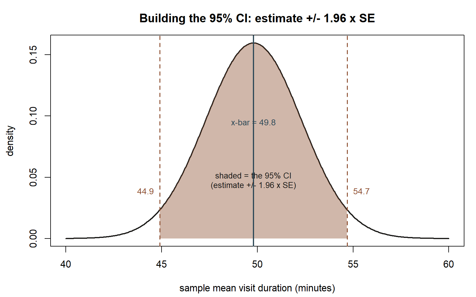
Recall the visit-duration sample from Weeks 2–3: n = 36 recorded MAC visits, sample mean x̄ = 49.8 minutes, and — using the known-σ teaching simplification (σ ≈ 15) — SE(x̄) = σ/√n = 15/6 = 2.5.
Symbolically:
\[ \bar{x} \;\pm\; 1.96 \cdot SE(\bar{x}). \]
Numerically:
\[ 49.8 \;\pm\; 1.96(2.5) \;=\; 49.8 \;\pm\; 4.9 \;=\; (44.9,\; 54.7). \]
Interpretation: if the MAC research team repeated this sampling process — draw n = 36 visits, compute x̄, build the interval x̄ ± 1.96·SE(x̄) — over and over, 95% of those intervals would contain the true mean visit duration μ. For this one sample, the interval happens to be (44.9, 54.7) minutes. You do not know whether this particular interval is one of the 95% that succeeded or one of the 5% that missed — you only know the procedure that generated it succeeds 95% of the time in the long run.
Worked example — MAC Study: a 95% CI for the usage rate
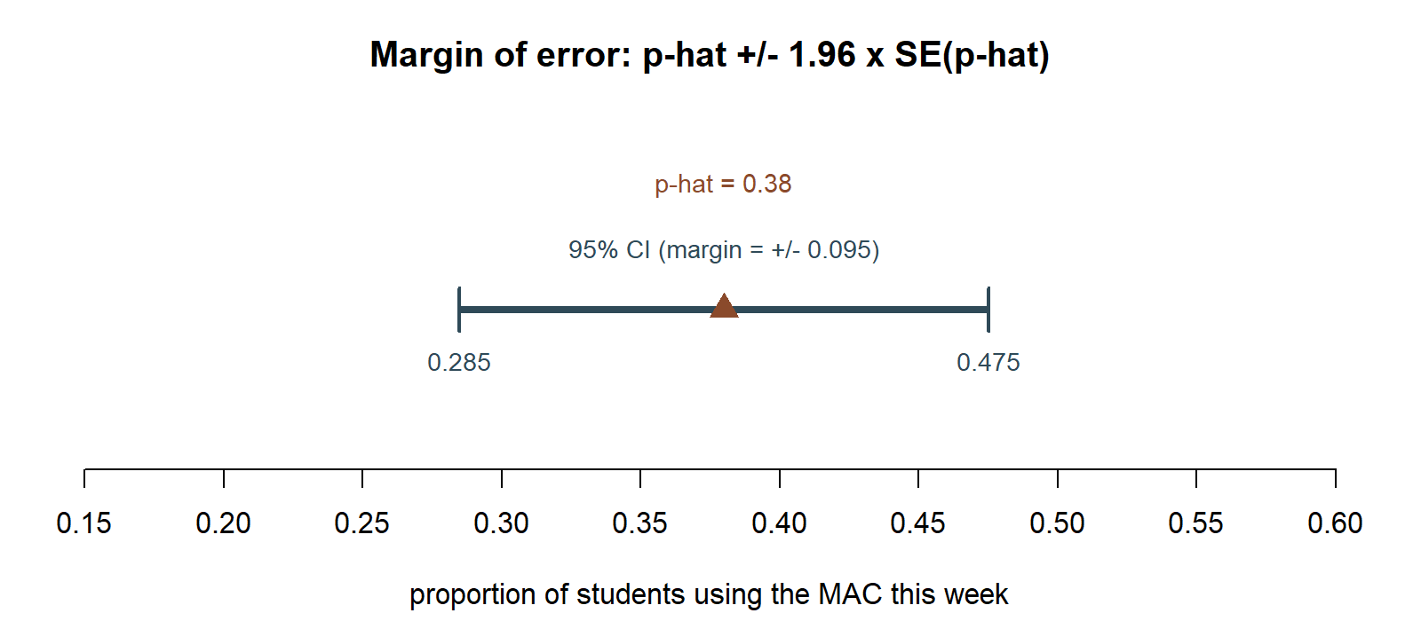
Recall the usage-rate survey: n = 100 students, k = 38 used the MAC at least once this week, p̂ = 0.38, and SE(p̂) = √(0.38 × 0.62 / 100) = √0.002356 ≈ 0.0485.
Symbolically:
\[ \hat{p} \;\pm\; 1.96 \cdot SE(\hat{p}). \]
Numerically:
\[ 0.38 \;\pm\; 1.96(0.0485) \;=\; 0.38 \;\pm\; 0.0951 \;=\; (0.285,\; 0.475). \]
Interpretation: the plausible range for the true proportion of students who use the MAC in a given week, at 95% confidence, runs from about 28.5% to 47.5%. That is a fairly wide interval — a reminder that even n = 100 leaves meaningful uncertainty about a proportion, especially one this close to the middle of the [0, 1] range where variability is largest.
This chunk is shown but not executed on this page (eval: false) — the figure below was produced by running exactly this computation separately (same seed, same formulas), reproduced as two number lines so you can check the chunk’s ci_mean and ci_prop output against a real result:
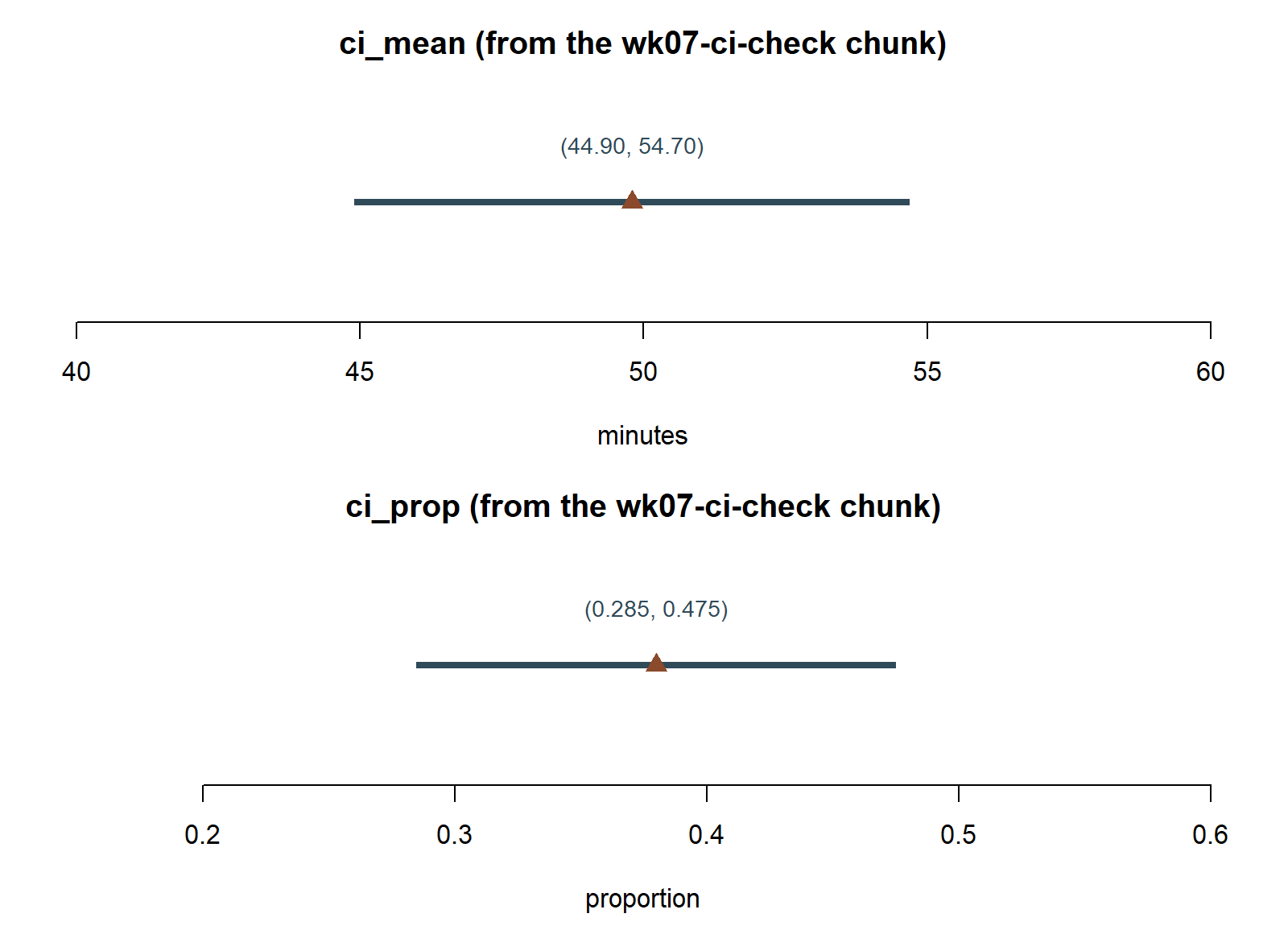
wk07-ci-check chunk above produces ci_mean = (44.90, 54.70) and ci_prop = (0.285, 0.475) — exactly the two intervals already worked out by hand above.
Worked example — transfer: average commute time at a different campus
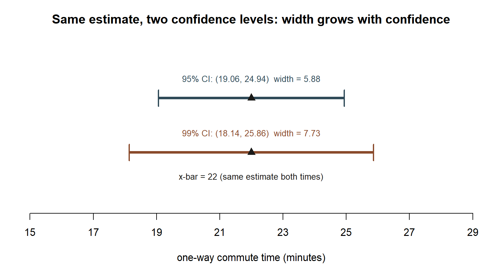
Synthetic; seed set. Suppose a different campus’s transportation office samples n = 49 students and asks how many minutes their one-way commute takes. The sample mean comes out to x̄ = 22 minutes, and (as a known-SD teaching simplification, mirroring the MAC Study’s approach) the population SD is treated as σ = 10.5 minutes, so SE(x̄) = σ/√n = 10.5/7 = 1.5.
Symbolically, the same recipe applies:
\[ \bar{x} \;\pm\; 1.96 \cdot SE(\bar{x}). \]
Numerically:
\[ 22 \;\pm\; 1.96(1.5) \;=\; 22 \;\pm\; 2.94 \;=\; (19.06,\; 24.94). \]
Interpretation: using this same procedure, the transportation office can report that they are 95% confident the true average one-way commute time for students at this campus lies between about 19.1 and 24.9 minutes — again, “95% confident” describing the long-run success rate of the method, not a probability attached to this one already-computed interval. Note that this is an entirely separate, synthetic campus and sample, invented only to give the same CI recipe a second context — it has no connection to the MAC Study numbers.
The same commute-time estimate also shows what “widening the confidence level” (from the general recipe, above) actually does to the interval: raising confidence from 95% to 99% keeps the point estimate fixed but uses the larger critical value z* ≈ 2.576 instead of 1.96, which widens the bracket.
A common mistake
The single most common CI misinterpretation: saying “there is a 95% probability that μ is in this specific interval (44.9, 54.7).” This sounds natural but is not what a frequentist confidence interval means. Once the sample is drawn and the numbers 44.9 and 54.7 are computed, there is nothing left to be random — μ either is or is not between those two numbers, full stop, and no probability statement attaches to that fixed fact. The 95% belongs to the procedure: if you imagine repeating the sampling-and-interval-building process many times, 95% of the resulting intervals (which will differ from sample to sample) would contain the true μ. It is correct to say “we used a procedure that captures the true parameter 95% of the time”; it is incorrect to say “there’s a 95% chance the true parameter is in this one interval we already built.” This is the same style of care needed with p-values (Week 8) — in both cases, the randomness lives in the sampling process, not in the fixed (if unknown) parameter or in one already-observed result.
Low-stakes self-checks (ungraded)
- Using the MAC usage-rate numbers, what would the 95% CI for π have been if the survey had used n = 400 instead of n = 100, with the same p̂ = 0.38? (Recompute SE(p̂) with the new n, then rebuild the interval.)
- True or false, and explain why: “If I built a 99% CI instead of a 95% CI for the same MAC visit-duration sample, the interval would be narrower.” (Think about what changes in the critical value.)
- In your own words, explain why the phrase “95% probability that μ is in this interval” is not a correct description of a confidence interval, using the repeated-sampling idea from this week.
- For the transfer example (commute times), what would the margin of error have been at 90% confidence instead of 95%? (You’ll need the 90% critical value, z* ≈ 1.645, applied to the same SE = 1.5.)
Reading and source pointer
This week’s spine is MIT OCW 18.05’s treatment of confidence intervals, which grounds the procedure-based derivation and interpretation used above. As an optional lighter pass, OpenIntro IMS’s chapter on confidence intervals for a mean and a proportion covers the same ground at a gentler pace and is worth a look if the 18.05 treatment moves too quickly. These notes are the course’s own synthesis, grounded in but not copied from the sources.
Public vs. graded
These notes, the examples, and the practice here are public and ungraded — study material only. No graded prompts, answer keys, rubrics, point values, or due dates appear on this site. Graded inference checkpoints, quizzes, homework, labs, the midterm, the project, and the final live in Blackboard (the LMS), which is authoritative for due dates, submissions, and grades. If this page and Blackboard ever disagree, follow Blackboard.
On the midterm specifically: the exam is Friday, Oct 9, in class, and covers first-half material — sampling distributions (Week 2) through confidence intervals (this week). Coverage details, format, and any review materials are posted in Blackboard, not here.
Looking ahead
Week 8 reuses this same standardized-distance idea — an estimate compared to a reference value, scaled by its standard error — but points it at a yes/no question instead of a range: is a specific hypothesized value of μ or π consistent with the data, or should it be rejected? The MAC Study’s visit-duration sample (x̄ = 49.8, SE = 2.5) returns immediately, tested against last year’s campus baseline of 45 minutes.