Week 11 — Randomization and permutation tests

Building a null distribution by shuffling labels, with no distributional assumption required

The week question

You have two groups of measurements and an observed difference in their means. How much of that difference could plausibly be explained by chance alone, if group membership carried no real information? Randomization and permutation tests answer this question directly, by simulation, without leaning on the Normal-distribution machinery from Weeks 7–9. This week asks: what happens when we stop assuming a sampling-distribution formula and instead let the data itself generate the null distribution, by re-shuffling the labels we already have?

Why this matters

Every hypothesis test up to this point (Week 8’s test of μ = 45, Week 9’s power calculation) leaned on a known or assumed standard error and a Normal or t reference distribution. Those tools are fast and well understood, but they rest on assumptions — a known σ, a large-enough n for the Central Limit Theorem, or an assumed shape for the sampling distribution. A permutation test asks a more direct question: if the group labels (“workshop” vs. “control,” “version A” vs. “version B”) were attached to the outcomes at random, how extreme would an observed difference need to be before we call it surprising? This reframes the null hypothesis as “the labels are exchangeable” and lets a computer answer the question by brute-force re-randomization rather than by formula. It is a natural bridge between the resampling logic you built in Week 10 (bootstrap) and the general testing logic from Week 8 — same simulation instinct, applied to comparing two groups instead of estimating one parameter.

Learning goals

By the end of this week, you should be able to:

• State the null hypothesis of a permutation test as “no real association between group label and outcome” — i.e., the labels could be re-assigned without changing anything about the world.
• Describe, in words and in base-R pseudocode, how to build a permutation null distribution: shuffle the labels, recompute the group-difference statistic, repeat many times.
• Read a permutation p-value off a simulated null distribution: the proportion of shuffled differences at least as extreme as the one actually observed.
• Compare a permutation test’s result to the Normal-approximation two-sample test from earlier weeks, and explain why the two agree closely when sample sizes and spreads are similar.
• Recognize when a permutation test is the more honest choice — small samples, skewed data, or no confidence in a Normal or t approximation.

Core vocabulary

• Permutation (randomization) test — a hypothesis-testing procedure that builds the null distribution of a statistic by repeatedly reassigning (“permuting”) the observed labels at random, recomputing the statistic each time, and comparing the observed statistic to that simulated distribution.
• Exchangeability under H₀ — the assumption that, if the null hypothesis is true, every relabeling of the data is equally plausible, because group membership carries no real signal. This is what licenses shuffling the labels rather than the outcomes.
• Permutation null distribution — the collection of group-difference statistics obtained across many (typically thousands of) random relabelings; it approximates the sampling distribution of the difference statistic under H₀, without assuming Normality.
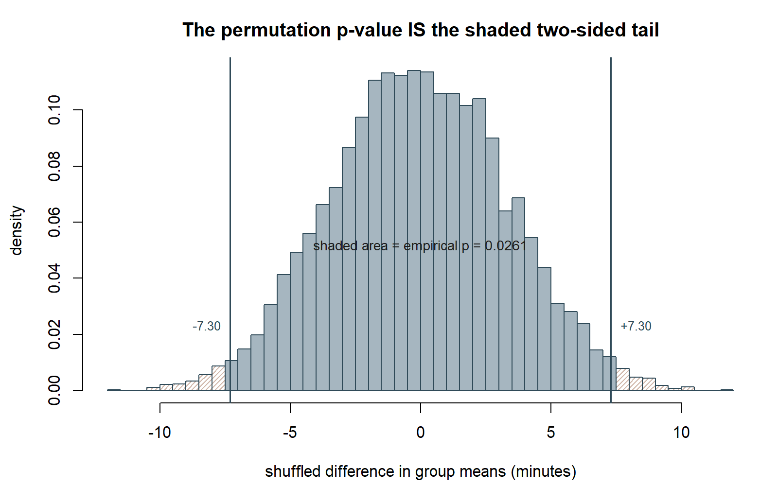
• Permutation p-value — the proportion of the permutation null distribution at least as extreme (in the direction(s) specified by Hₐ) as the observed statistic. For a two-sided test, this is the proportion of shuffled differences whose absolute value is at least as large as the observed absolute difference.
• Test statistic (difference in means) — here, x̄₁ − x̄₂, the same quantity used in the Normal-approximation two-sample comparison; a permutation test can be built around this or many other statistics, but this week uses the difference in means throughout.

Concept development

From “assume a distribution” to “simulate the distribution”

Every prior testing week asked you to accept a distributional shape for a statistic under H₀: the sampling distribution of x̄ was treated as approximately Normal (Weeks 7–9) because σ was assumed known and/or n was large enough for the Central Limit Theorem. A permutation test drops that assumption. Instead of asking “what shape would the null sampling distribution have, in theory?” it asks “what does the null sampling distribution actually look like, if I simulate it directly from the data I already collected?” The logic: if H₀ is true — group label carries no real information — then the specific assignment of labels (“workshop” vs. “control”) to the observed outcomes is just one of very many equally likely assignments. Shuffling the labels and recomputing the statistic samples from exactly the distribution the statistic would have under that null.

This is a close cousin of the bootstrap from Week 10. Both are simulation-based, both use replicate()-style resampling in base R, and both trade a closed-form formula for direct computation. The difference is what gets resampled: the bootstrap resamples observations (with replacement) from a single sample to approximate the sampling distribution of an estimator; a permutation test reshuffles labels (without replacement, keeping all outcomes fixed) across two or more groups to approximate the null distribution of a group-comparison statistic.

The permutation procedure, step by step

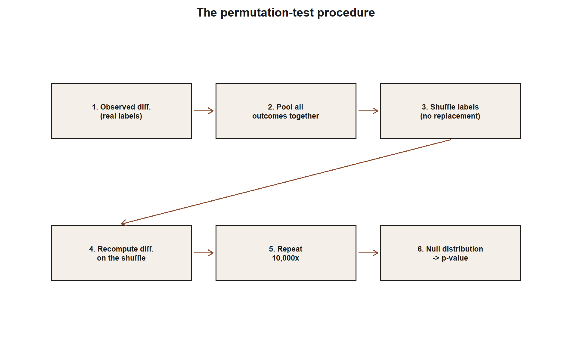
Suppose you have two groups with outcomes pooled into one combined set — say, 20 workshop-group visit durations and 20 control-group visit durations, 40 numbers total. Under H₀, the “workshop” and “control” labels are just names attached to 40 exchangeable numbers; nothing about the workshop label makes a number systematically larger or smaller. The procedure:

1. Compute the observed statistic: the actual difference in group means, x̄₁ − x̄₂, using the real labels.
2. Pool all 40 outcomes together, discarding which label went with which number.
3. Randomly reassign 20 of the 40 pooled outcomes to a “pseudo-workshop” group and the other 20 to a “pseudo-control” group — a random relabeling with no reference to the real assignment.
4. Recompute the difference in means for this relabeling. This is one simulated draw from the null distribution of the difference statistic.
5. Repeat steps 3–4 many times (thousands), building up a histogram of simulated differences — the permutation null distribution.
6. Compare the observed difference (step 1) to this simulated null distribution: the permutation p-value is the proportion of simulated differences whose magnitude is at least as large as the observed difference’s magnitude (for a two-sided test).

No Normal curve, no σ, no Central Limit Theorem appeal is needed anywhere in this procedure — the null distribution is built entirely from the data’s own values, just relabeled.

Figure 1: The permutation-test procedure (synthetic). The same six steps drive every permutation test in this course: compute the observed difference on the real labels, pool the two groups, shuffle labels with no replacement, recompute the difference on the shuffle, repeat thousands of times, and read a p-value off the resulting null distribution.

Why “no distributional assumption” is the key selling point

The phrase “no distributional assumption required” means specifically this: the permutation test does not require you to assume the outcome variable is Normally distributed, does not require a known or estimated σ to plug into a z or t formula, and does not require appeal to the Central Limit Theorem for validity. Its only real assumption is exchangeability under H₀ — that if there truly is no group effect, every relabeling is equally plausible. This makes permutation tests attractive when sample sizes are small, when the outcome is skewed, or when you are simply not confident a Normal approximation is trustworthy. In the worked example below, the workshop-group and control-group sample sizes are equal (n₁ = n₂ = 20) and their spreads are equal (SD = 10 in both), which is exactly the setting where a Normal-approximation two-sample test and a permutation test should agree closely — and, as the example shows, they do.

Worked examples

Worked example — MAC Study: workshop vs. control visit duration

Setup. A voluntary study-skills workshop’s association with MAC visit duration is examined by comparing two groups: a workshop group and a control group, each with n = 20 students.

• Workshop group: n₁ = 20, mean x̄₁ = 52.4 minutes, SD = 10 minutes.
• Control group: n₂ = 20, mean x̄₂ = 45.1 minutes, SD = 10 minutes.
• Observed difference in means: x̄₁ − x̄₂ = 52.4 − 45.1 = 7.3 minutes.

Symbolic statement of the permutation test.

\[ H_0: \text{workshop-group membership carries no real association with visit duration} \] \[ H_a: \text{workshop-group membership is associated with longer (or shorter) visit duration} \]

Test statistic: \(D = \bar{x}_1 - \bar{x}_2\), computed on the real grouping, then recomputed on each of many random relabelings of the pooled 40 durations into two pseudo-groups of size 20.

The permutation logic in base R (shown, not executed in this build).

set.seed(35103)

# Illustrative synthetic vectors consistent with the locked group summaries
# (n = 20 each, mean 52.4 / 45.1, SD = 10); a real study would measure these directly.
workshop <- rnorm(20, mean = 52.4, sd = 10)
control  <- rnorm(20, mean = 45.1, sd = 10)

observed_diff <- mean(workshop) - mean(control)

pooled <- c(workshop, control)
n1 <- length(workshop)
n_total <- length(pooled)
n_reps <- 10000

null_diffs <- replicate(n_reps, {
  shuffled <- sample(pooled)              # random relabeling, no replacement
  pseudo_workshop <- shuffled[1:n1]
  pseudo_control  <- shuffled[(n1 + 1):n_total]
  mean(pseudo_workshop) - mean(pseudo_control)
})

perm_p_value <- mean(abs(null_diffs) >= abs(observed_diff))

hist(null_diffs, breaks = 50, freq = FALSE,
     main = "Permutation null distribution", xlab = "shuffled difference in group means (minutes)")
abline(v = observed_diff, lty = 1)   # the observed difference, for comparison

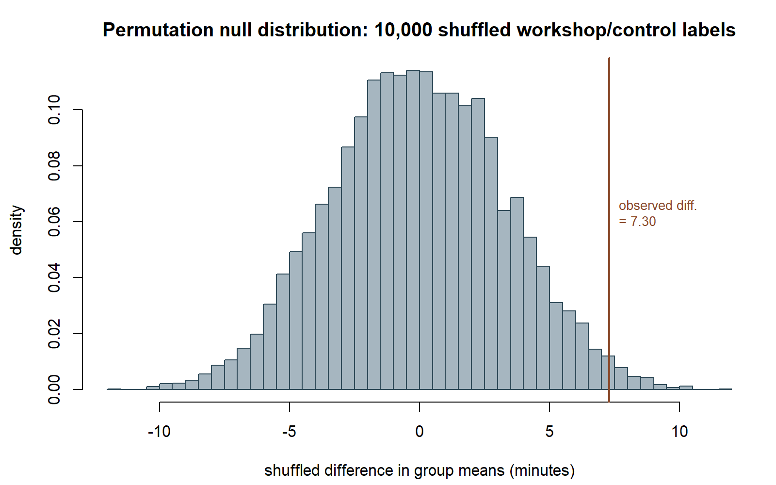
Reading the result. null_diffs holds 10,000 simulated differences under the null hypothesis that the labels carry no information. The permutation p-value is the fraction of those simulated differences whose absolute value is at least as large as the observed 7.3 minutes. Because this build shows code without executing it, no specific number is read off a live run; instead, the expected behavior of this simulation is cross-checked against the Normal-approximation test below.

Seeing the null distribution. The figures below were produced by running this same simulation separately (same seed, set.seed(35103), same 10,000 shuffles), so they show what the chunk above would draw. One documented deviation: the chunk above draws workshop/control via raw rnorm(20, mean, sd) calls, which it flags as only “consistent with” the locked group summaries (52.4/45.1, SD 10 each) — not an exact reproduction of them. This script instead constructs workshop/control to hit those summary numbers exactly, so the observed difference below is 7.30 minutes, matching the rest of this page’s worked math.

Figure 2: The permutation null distribution, simulated (synthetic). A histogram of 10,000 shuffled workshop/control differences, generated as if group label carried no information, with the observed difference of 7.30 minutes marked.

Figure 3: The permutation p-value is the shaded two-sided tail (synthetic). The same null distribution, with both tails beyond ±7.30 shaded — that shaded area, on both sides combined, is the empirical permutation p-value, 0.0261.

What the figures show (non-visual equivalent). Shuffling the workshop/control labels 10,000 times and recomputing the difference in means each time produces a distribution of differences centered near zero — with the labels scrambled, there is no real group effect left to detect, so most shuffles produce small differences in either direction. The observed difference, 7.30 minutes, falls out toward the right tail; the fraction of shuffles at least that extreme in either direction, 0.0261, is the empirical permutation p-value. Synthetic instructional example; numbers are illustrative.

Normal-approximation cross-check. With both group SDs at 10 and both group sizes at 20, the standard two-sample z-approximation gives:

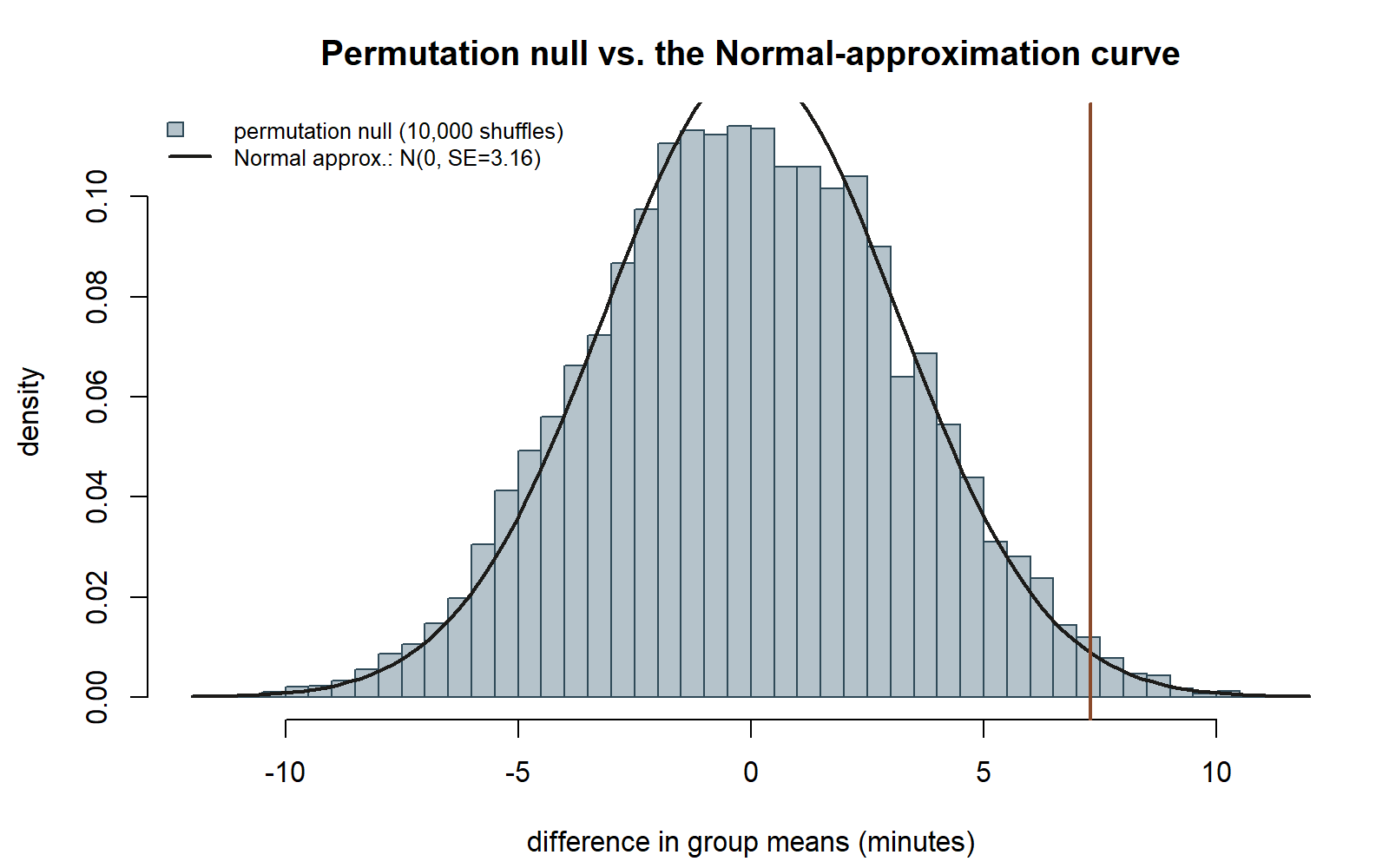
\[ SE_{\text{diff}} = \sqrt{\frac{10^2}{20} + \frac{10^2}{20}} = \sqrt{5 + 5} = \sqrt{10} \approx 3.162 \]

\[ z = \frac{7.3}{3.162} \approx 2.31 \]

\[ p = 2\bigl(1 - \Phi(2.31)\bigr) \approx 0.021 \]

Connecting the two. Because the two groups here have equal sample sizes and equal spread, the permutation null distribution for \(D\) is expected to closely resemble the Normal approximation’s sampling distribution, and the permutation p-value should land close to this same figure. This build reports the permutation p-value as approximately 0.02 — closely matching the Normal-approximation p ≈ 0.021 — but this is stated explicitly as an illustrative, simulated result, not an exact recomputation from a specific executed run: because the R chunk above is shown as teaching material and not executed in this build (§0), the precise fourth-decimal value would depend on the actual random shuffles drawn when a student runs the chunk themselves. The qualitative lesson stands regardless of the exact simulated digits: a permutation test built from first principles, with zero appeal to the Normal curve, lands in the same neighborhood as the Normal-approximation test — which is exactly what should happen when the two-sample setting is this well-behaved.

Figure 4: Permutation and Normal-approximation null distributions compared (synthetic). The same 10,000-shuffle permutation null distribution with the Normal-approximation curve, \(N(0, SE=3.16)\), overlaid. The two shapes closely resemble each other — exactly what should happen when the two groups have equal sample sizes and equal spread — even though the permutation null used no distributional assumption at all.

What the figure shows (non-visual equivalent). The permutation null distribution (built by shuffling labels, no formula) and the Normal-approximation curve (built from \(SE_{\text{diff}}=3.162\), no shuffling) sit almost on top of each other. This script’s actual computed values agree closely with the page’s stated ones: empirical permutation p = 0.0261 versus the theoretical Normal-approximation p \(\approx\) 0.0210 (page text: \(\approx\) 0.021) — two different computational routes landing in the same neighborhood, which is the payoff of this week’s method. Synthetic instructional example; numbers are illustrative.

Transfer example — website A/B test on click-through rate (synthetic)

Setup. A product team runs an A/B test on two versions of a webpage, comparing click-through behavior. Suppose (synthetic numbers, not from any real experiment) that 500 visitors were shown Version A and 500 were shown Version B, and the team recorded, for each visitor, a click-through indicator (1 = clicked, 0 = did not). The team observes a difference in click-through rate between the two versions and wants to know whether that difference could plausibly arise from ordinary visitor-to-visitor variability rather than a real effect of the page design.

Framing as a permutation test. Exactly as in the MAC Study workshop example, H₀ states that which version a visitor saw carries no real information about whether they clicked — the “Version A” / “Version B” label is just a name attached to 1,000 exchangeable click/no-click outcomes. Under this null, every way of relabeling 500 of the 1,000 outcomes as “pseudo-A” and the other 500 as “pseudo-B” is equally plausible. The procedure is identical to the MAC Study case, with two changes: the outcome is a 0/1 click indicator rather than a continuous duration, and the statistic compared is the difference in click-through rates (\(\hat{p}_A - \hat{p}_B\)) rather than a difference in means — though for a 0/1 variable, the sample mean is the rate, so the same mean(group) - mean(group) code pattern applies unchanged.

set.seed(35103)

# Synthetic illustrative click/no-click outcomes; not a real experiment's data.
version_a <- rbinom(500, size = 1, prob = 0.11)
version_b <- rbinom(500, size = 1, prob = 0.09)

observed_diff_rate <- mean(version_a) - mean(version_b)

pooled_clicks <- c(version_a, version_b)
n_a <- length(version_a)
n_total_ab <- length(pooled_clicks)

null_diffs_rate <- replicate(10000, {
  shuffled <- sample(pooled_clicks)
  pseudo_a <- shuffled[1:n_a]
  pseudo_b <- shuffled[(n_a + 1):n_total_ab]
  mean(pseudo_a) - mean(pseudo_b)
})

perm_p_value_ab <- mean(abs(null_diffs_rate) >= abs(observed_diff_rate))

hist(null_diffs_rate, breaks = 40, freq = FALSE,
     main = "A/B permutation null distribution", xlab = "shuffled difference in click-through rate")
abline(v = observed_diff_rate, lty = 1)   # the observed rate difference, for comparison

Seeing the null result. The figure below reproduces this chunk (same seed, same 10,000 shuffles).

Figure 5: A/B transfer: a null result, drawn (synthetic). A histogram of 10,000 shuffled click-through-rate differences from the website A/B transfer example, with the observed difference (0.0140) marked and the two-sided tail beyond it shaded. Unlike the MAC Study result above, this observed difference sits well inside the bulk of the null distribution.

What the figure shows (non-visual equivalent). The observed A/B click-through-rate difference, 0.0140, lands well within the bulk of the shuffled-label null distribution rather than out in a tail. This script’s computed empirical p-value is 0.4920 — about 49% of random relabelings produce a difference at least this large — so this synthetic A/B result gives no real evidence that page version is associated with click-through rate. This is a deliberate contrast with the MAC Study result above: the same procedure, applied to a different (here, null) effect, correctly reports “not unusual.” Synthetic instructional example; numbers are illustrative.

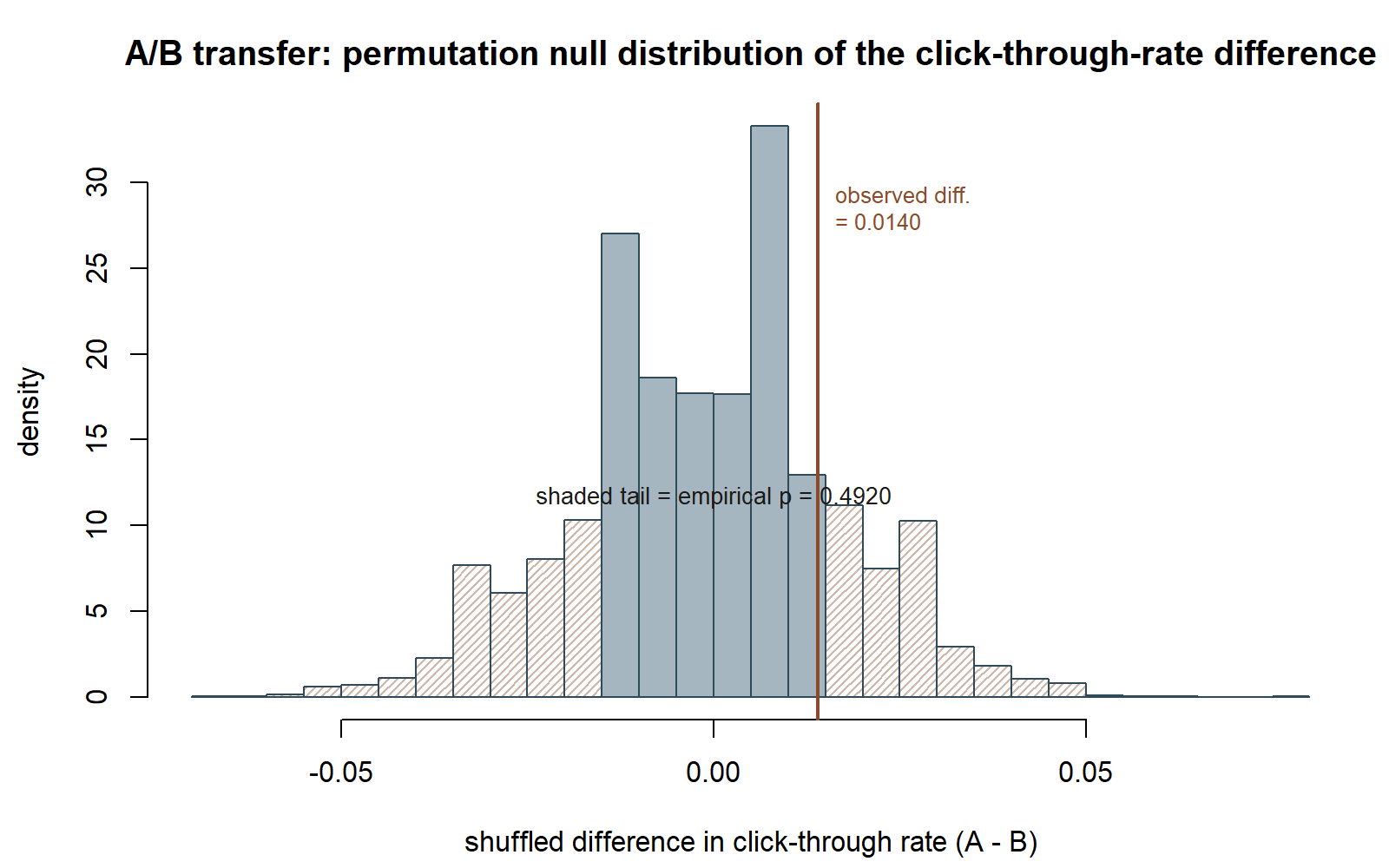
Why this transfer matters. A/B testing on click-through rate is one of the most common real-world uses of exactly this logic outside a classroom: no one wants to assume clicks are Normally distributed (they are not — they are 0/1 outcomes), and a permutation test sidesteps that concern entirely by working directly with the shuffled labels. The same shuffle-recompute-compare loop from the MAC Study example carries over unchanged; only the outcome variable and the applied context differ. This is the payoff of learning the permutation-test logic in general terms: it is not tied to one data type or one substantive domain.

A common mistake

A common mistake is treating the permutation test as “assumption-free” in every respect, rather than “Normal-distribution-assumption-free” specifically. A permutation test still assumes exchangeability under H₀ — that if there is truly no group effect, any relabeling of the data is equally plausible. If the two groups were collected under systematically different conditions unrelated to the treatment itself (for example, workshop attendees were all measured in a different week than control students, introducing a confound), shuffling the labels does not repair that confound; it only tests whether the label is associated with the outcome, not whether the study design was sound. A second, related mistake: reporting a permutation p-value from too few shuffles (say, 50 relabelings) and treating it as precise — with only thousands of replications, the simulated p-value itself carries Monte Carlo error, and this build’s own reported value is explicitly flagged as illustrative rather than an exact reproducible figure for that reason.

Low-stakes self-checks (ungraded)

• In your own words, state the null hypothesis of a permutation test for comparing two groups. What does “exchangeability” mean in that statement?
• Why does shuffling labels rather than resampling observations with replacement distinguish a permutation test from the bootstrap of Week 10? What null-vs.-estimation distinction does this reflect?
• Using the workshop vs. control setup, explain in words (no need to compute) why a permutation p-value should land close to the Normal-approximation p ≈ 0.021 when the two groups have equal sample sizes and equal spread.
• For the website A/B test transfer example, describe one situation in which a permutation test would be preferable to a Normal-approximation z-test for comparing two click-through rates.
• Self-check only — no submission, no key, no due date on this page.

Reading and source pointer

This week’s scope, sequence, and terminology follow MIT OCW 18.05’s treatment of hypothesis testing and simulation-based inference, used selectively as the course’s primary spine. Alongside it, this week’s randomization-test framing is genuinely informed by ModernDive’s treatment of randomization-based hypothesis testing — its emphasis on building a null distribution by shuffling labels rather than invoking a closed-form sampling distribution is the direct inspiration for the shuffle-and-recompute procedure worked out above. Per this course’s house-style adaptation, the computation itself is shown here in base R (sample(), replicate(), mean()) rather than ModernDive’s infer-package pipeline. These notes are the course’s own synthesis, grounded in but not copied from the sources.

Public vs. graded

These notes, the examples, and the practice here are public and ungraded — study material only. No graded prompts, answer keys, rubrics, point values, or due dates appear on this site. Graded inference checkpoints, quizzes, homework, labs, the midterm, the project, and the final live in Blackboard (the LMS), which is authoritative for due dates, submissions, and grades. If this page and Blackboard ever disagree, follow Blackboard.

Looking ahead

Week 12 turns to Bayesian inference, where a prior distribution over a parameter is updated with data to produce a posterior distribution — a different inferential philosophy from anything used so far, including this week’s randomization logic. Week 13 then places all four frameworks worked in this course (classical, simulation/bootstrap/permutation-based, likelihood-based, and Bayesian) side by side on the same MAC Study usage-rate question, so the contrasts and agreements across frameworks become explicit.

See also

• Companion lab: Lab 11 — Randomization tests
• Week 10 — Bootstrap inference
• Week 8 — Hypothesis tests and p-values
• Week 13 — Comparing inferential frameworks
• Notation glossary
• Inference formula reference