Week 11 — Simulation-based inference

MATH 21003 · Introduction to Statistical Methods · Fall 2026 · Week 11 (Nov 2–6, 2026)

Why this week matters

For ten weeks we have described data and built models — means, proportions, tables, regression lines. Every one of those summaries was a number computed from a sample. This week we finally ask the two questions that turn a sample into a conclusion about the world: could this pattern be due to chance alone? and what values are plausible for the real quantity? Those are the questions of statistical inference, and back in Week 9 we deliberately left them open: when we read a regression output we covered the “Std. Error / t / p” columns in grey and labeled them “Weeks 11–12.” This is Week 11. We are about to fill in what those columns answer.

The honest way to learn inference is to watch it happen before you trust a formula for it, so this week we answer both questions by simulation — letting the computer act out “pure chance” thousands of times and seeing where the real data fall. The in-class tool is StatKey; you will read its plots, not write any code. The rhythm: Monday builds the chance model — an observed statistic, a null of “no effect,” and a null distribution. Wednesday runs StatKey for both a randomization test and a bootstrap, and practices reading the output. Friday focuses on meaning: a p-value as strength of evidence, and a confidence interval as a range of plausible values.

Monday: the logic of a randomization test

Start with a real question. In a 1970s study of possible sex discrimination, 48 supervisors each reviewed a personnel file and decided whether to promote. The files were identical except for a name indicating sex, and they were randomly assigned. Among the 24 “male” files, 21 were promoted (\(21/24 = 0.875\)); among the 24 “female” files, 14 were promoted (\(14/24 = 0.583\)). The gap — the observed statistic — is

\[\frac{21}{24} - \frac{14}{24} = 0.292,\]

a 29.2 percentage-point difference favoring the male files. The question is not “is there a gap?” — there plainly is one in this sample — but could a gap this big show up just from the luck of which files landed in which pile, even if sex made no difference at all?

To answer it we set up a chance model. The null hypothesis is the skeptic’s position: sex has no effect on the promotion decision. If that were true, the 35 “promote” decisions and 13 “do not promote” decisions were going to come out the way they did regardless of the name on the file — so we can shuffle the labels and redeal them. Each shuffle is a world in which the null is true, and each gives a new difference in promotion rates. Do this many times and you get a null distribution: the collection of differences you would expect from chance alone. It is centered at zero (no effect) and shows how big a gap chance typically produces. For the discrimination study, 100 simulated shuffles almost never reached the real 29.2-point gap — only about 2 of the 100 did — which already tells us the observed gap is hard to explain as luck.

The recipe is the same every time, so it is worth naming:

Identify the observed statistic (here, the difference in promotion rates, \(0.292\)).
State the null — “no effect / no difference” — as the chance model.
Simulate under that model many times (shuffle and recompute).
Build the null distribution of the simulated statistics.
See how unusual the observed statistic looks against it.

Wednesday, part 1: reading a null distribution and a p-value

Wednesday we run this in StatKey. Take the chunk’s main example, the opportunity-cost study (it returns next week, so keep it in mind). Students were asked whether to buy a video; one group was first reminded that keeping the money was an option. Of 75 in the control group, 19 chose not to buy (\(0.253\)); of 75 reminded students, 34 chose not to buy (\(0.453\)). The observed statistic is

\[\frac{34}{75} - \frac{19}{75} = 0.200,\]

a 20-point increase in “did not buy.” Could the reminder be doing nothing, with a 20-point gap arising by chance? StatKey shuffles the 53 “not buy” decisions across the two groups 1,000 times and plots the null distribution:

A histogram of 1,000 simulated differences in proportions, centered at zero and roughly bell-shaped, ranging from about negative 0.3 to positive 0.3. A vertical red line at 0.20 is labeled observed 0.20 and sits in the far right tail. A small shaded region at and beyond 0.20 is annotated that 6 of 1,000 simulations landed there. Text notes the p-value is 6 divided by 1,000, about 0.006. — A StatKey-style null distribution for the opportunity-cost study: a histogram of 1,000 simulated differences in the proportion who did not buy, assuming the reminder had no effect. The histogram is bell-shaped and centered at zero. A red line marks the observed difference of 0.20 far out in the right tail; only 6 of the 1,000 simulations reached 0.20 or beyond, so the simulated p-value is about 0.006.

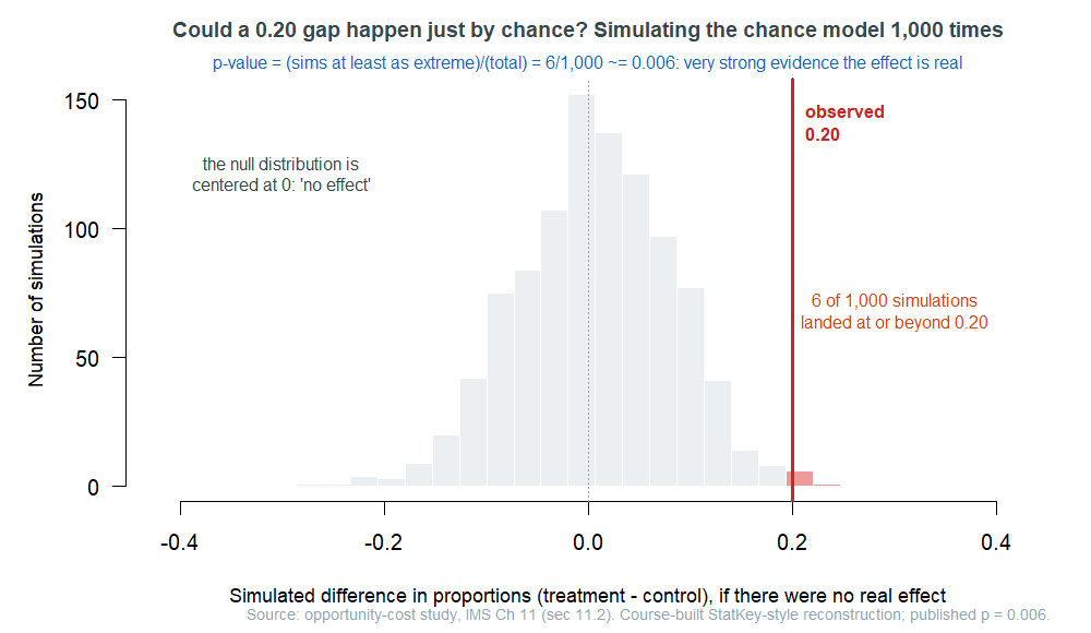
Now read the p-value. It is simply the fraction of the null distribution that is at least as extreme as what we saw: here, \(6\) of the \(1{,}000\) simulated gaps reached \(0.20\) or more, so

\[p\text{-value} = \frac{6}{1{,}000} = 0.006.\]

A p-value answers one question: if the null were true, how often would chance alone produce data as extreme as ours? A small p-value means “rarely” — our data would be a surprise in a world of no effect — and so it is evidence against the null. The traditional language calls a result statistically significant when the p-value falls below a chosen significance level (often \(0.05\)); IMS sometimes calls the same idea statistical discernibility, but we will say significant. At \(p = 0.006\) the opportunity-cost effect is significant: strong evidence that the reminder really does change behavior.

Two cautions that we will keep all week. First, the court analogy: a trial starts by presuming innocence (the null) and asks whether the evidence is strong enough to reject it. A small p-value is like strong evidence of guilt; a large p-value is failure to convict, which is not the same as proving innocence. “Fail to reject the null” never means “the null is true” — only that this study did not find enough evidence against it. Second, a p-value is not the probability that the null is true; it is a probability computed assuming the null is true.

Wednesday, part 2: bootstrapping for a range of plausible values

A p-value answers “could it be chance?” The other question is “how big is the effect, really?” — and for that we want an interval of believable values. We get one by bootstrapping.

The idea is almost cheeky. We only have one sample, but it is our best picture of the population, so we treat the sample as a stand-in for the population and draw new samples from it — sampling with replacement, so a given observation can appear more than once or not at all. Each such resample is the same size as the original and gives a slightly different statistic. Collect thousands of them and you get a bootstrap distribution: a picture of how much the statistic would wobble from sample to sample.

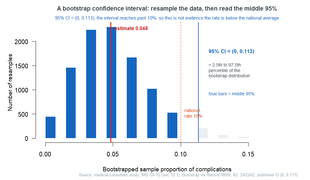
Consider the medical-consultant case (it, too, returns next week). A consultant claims her clients have fewer surgical complications than the national rate of about \(10\%\). Among her \(62\) clients, \(3\) had a complication, a rate of \(\hat p = 3/62 = 0.048\) — about half the national figure. But \(62\) is a small sample; how seriously should we take \(0.048\)? StatKey resamples those 62 outcomes 10,000 times and plots the bootstrap distribution of the proportion:

A histogram of 10,000 bootstrapped sample proportions ranging from 0 to about 0.15, roughly bell-shaped with a slight right skew. A red vertical line marks the estimate 0.048. Most bars are shaded blue to show the middle 95 percent. A blue vertical line at 0.113 marks the 97.5th percentile and the left edge at 0 marks the 2.5th percentile. A dashed amber line at 0.10 is labeled national rate 10 percent. A side note reads 95 percent CI equals 0 to 0.113. — A bootstrap distribution for the medical-consultant study: a histogram of 10,000 bootstrapped complication proportions from a sample of 62 with 3 complications. The estimate of 0.048 is marked. The middle 95 percent of the distribution, shaded blue, runs from the 2.5th percentile at 0 to the 97.5th percentile at 0.113, so the 95 percent confidence interval is 0 to 0.113. A dashed line marks the national rate of 10 percent, which falls inside the interval.

Friday: confidence intervals as plausible values, read honestly

To turn that bootstrap distribution into a confidence interval, we use the percentile rule: for a 95% interval, chop off the bottom \(2.5\%\) and the top \(2.5\%\) and keep the middle 95%. For the consultant, the 2.5th percentile is \(0\) and the 97.5th percentile is \(0.113\), so the

\[95\% \text{ confidence interval} = (0,\ 0.113).\]

Read it as a range of plausible values for her true complication rate: anything from \(0\%\) up to about \(11.3\%\) is consistent with her data. Crucially, the national rate of \(10\%\) falls inside that interval — so despite the eye-catching \(0.048\), this is not convincing evidence that her rate is below average. The interval is honest about how little 62 surgeries can pin down. (A wider net catches the truth more often but tells you less; a 99% interval would be wider, a 90% one narrower. More data tightens the net.)

A confidence interval is only useful if you read it correctly, and most people don’t. Here is the careful version next to the two classic misreadings:

A two-column schematic. The left green column headed What it DOES mean explains that a 95 percent confidence interval is a range of plausible values for the parameter, that 95 percent of intervals built this way capture the true value in the long run with about 1 in 20 missing, and that the national rate stays plausible because the interval reaches past 10 percent. The right red column headed What it does NOT mean lists three crossed-out misreadings: a 95 percent chance the true value is in this interval, 95 percent of the data falling inside, and the interval proving the rate is zero. — A two-panel schematic titled Reading a 95 percent confidence interval honestly for the medical-consultant interval 0 to 0.113. The left green panel, What it DOES mean, says the interval is a range of plausible values for the true rate, built so that in the long run 95 percent of such intervals capture the true value, and that because the interval reaches past 10 percent the national rate stays plausible. The right red panel, What it does NOT mean, marks three wrong readings: that there is a 95 percent chance the true rate is inside this particular interval, that 95 percent of the data fall in the interval, and that the interval proves the rate is zero.

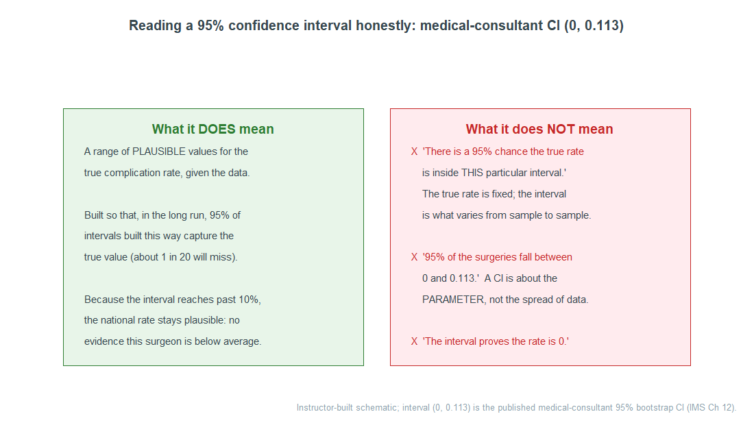
The single most common error is to say “there is a \(95\%\) chance the true rate is between \(0\) and \(0.113\).” But the true rate is a fixed (unknown) number — it is either in this interval or it isn’t. What varies from sample to sample is the interval. The right statement is about the procedure: if we repeated the whole study many times, about \(95\%\) of the intervals we built this way would contain the true value. That is why we say we are “\(95\%\) confident,” not “\(95\%\) probable.”

This is the week’s caution habit, the same one we have practiced since Week 2 — the number is not the whole story. A p-value is evidence, not proof. “Fail to reject” is not “accept.” A confidence interval is a statement about plausible values for the parameter, not about \(95\%\) of the data. And statistical significance is not practical importance: a tiny, unimportant effect can be significant with enough data, and an important one can go undetected with too little.

Common mistakes

“The p-value is the probability the null is true.” No. It is the probability of data this extreme if the null is true — a very different conditional. (\(p = 0.006\) does not mean a \(0.6\%\) chance of no effect.)
“A big p-value proves there is no effect.” It only means this study did not find convincing evidence of one. Fail to reject ≠ accept the null.
“95% of the data fall in the confidence interval.” A CI is about the parameter (the true rate or mean), not the spread of individual observations.
“There’s a 95% chance the true value is in this interval.” The true value is fixed; the interval is what’s random. The 95% is a property of the method over many samples.
“Bootstrapping invents new data.” It only resamples the data you already have, with replacement, to see how much your statistic would wobble. It adds no new information — it reveals the uncertainty already there.
“Significant means important.” Statistical significance is about ruling out chance, not about the size or real-world weight of an effect.

What you should be able to do by Friday

By the end of Week 11 you should be able to:

identify the observed statistic and state the null hypothesis (“no effect / no difference”) for a study;
explain what a null distribution represents and why it is centered at the null value;
read a p-value off a simulated null distribution as the fraction at least as extreme as the observed statistic, and interpret it as strength of evidence;
explain bootstrapping as resampling-with-replacement from the sample, and what a bootstrap distribution shows;
read a 95% confidence interval off a bootstrap distribution using the percentile rule, and interpret it as a range of plausible values;
avoid the ritual misreadings: p-value ≠ P(null true), fail-to-reject ≠ accept, CI ≠ “95% of the data,” and significant ≠ important.

Assignments this week

Monday check. A short in-class concept check on identifying the observed statistic and the null, and on what a null distribution represents. Plan for about 3–5 minutes. Sheet: Week 11 Monday exit ticket.
Wednesday check. A short application reading a StatKey output — a null distribution or a bootstrap distribution — and interpreting the p-value or the percentile interval. Plan for about 8–12 minutes. Sheet: Week 11 Wednesday exit ticket.
🔒 Friday quiz — handled through Blackboard or in class as directed. The quiz prompt is not posted here. Timing and submission details live in Blackboard.
🔒 Homework 6 (biweekly, Weeks 11–12) — posted and submitted through Blackboard. It spans this week and next; the simulation half is due alongside the classical half after Week 12.

Reuse

CC BY-SA 3.0.