Week 2 — Study design, bias, and causality

MATH 21003 · Introduction to Statistical Methods · Fall 2026 · Week 2 (Aug 31 – Sep 4, 2026)

Why this week matters

Last week we said statistics starts when you can read a dataset. This week we go one question earlier: how were these data collected?

The answer matters more than the headline ever suggests. The same headline number — “patients on this drug had a stroke 20% of the time” — can be strong evidence, weak evidence, or no evidence at all, depending on how the data underneath were collected. A randomized trial of 451 patients tells you one thing. A retrospective chart review of a self-selected group tells you something very different. By Friday you should be able to look at a short study description and judge, honestly:

Who or what does this study actually generalize to?
Was this an experiment or an observational study?
Are causal claims here defensible?
What else could explain what we see?

The point is simple: before we interpret a result, we need to know how the data were collected. Read the design before trusting the claim — it’s the habit everything else in the course passes through.

Populations, samples, and study claims

Every study has a population in mind — the full group of cases the research question is really about. Three examples:

Research question	Population (what the study is really about)
What is the average mercury content in swordfish in the Atlantic Ocean?	All swordfish in the Atlantic Ocean.
Over the last five years, what is the average time to complete a degree for our university’s undergraduates?	All recent undergraduates at our university who finished a degree.
Does a new drug reduce the rate of deaths in patients with severe heart disease?	All patients with severe heart disease (or some clearly described subset of them).

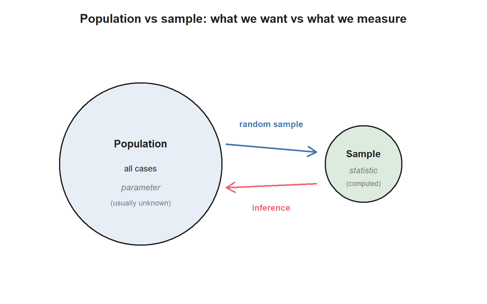
In practice, no one measures the entire population. Researchers collect a sample — a small fraction of the population they can actually observe. The summary numbers they compute from a sample are called sample statistics. The corresponding numbers we would get if we measured the whole population are called population parameters. Sample statistics are our best guess at population parameters; they are not the same thing.

You’ll see these four words a lot this term:

Population — what the question is about.
Sample — who or what we actually measured.
Parameter — a number describing the population (usually unknown).
Statistic — a number describing the sample (always computable from data).

Schematic showing a large population circle, a random-sample arrow to a small sample circle, and an inference arrow back to the population. — We almost never measure the whole population. We draw a random sample, compute a statistic, and use it to infer the unknown population parameter.

Sampling and representativeness

A sample is useful only if it looks like the population it’s meant to represent. If the sample is built in a way that systematically leaves people out, or systematically over-counts a particular group, it is biased — and analysis on a biased sample can mislead you even if every individual measurement is perfect.

The cleanest way to avoid sample bias is random sampling: every case in the population has the same chance of being chosen. The simplest version is called a simple random sample (SRS): imagine writing every patient’s name on a card and pulling cards out of a hat at random. The US Centers for Disease Control runs a real example — the Behavioral Risk Factor Surveillance System (BRFSS) — which conducts over 400,000 telephone interviews per year using a randomized procedure. That’s how we get population-level estimates about smoking, exercise, and chronic conditions.

A few traps to watch for:

Convenience sampling. Asking the patients who are easiest to reach. Easy to do; almost always biased. (If you survey only the patients in the waiting room, you are not surveying the patients who don’t need to be in the waiting room.)
Voluntary response. Letting respondents self-select into the sample. People with strong feelings are over-represented.
Non-response bias. Some people you tried to reach didn’t respond. If non-responders differ systematically from responders, your data are skewed.

You’ll see two more sampling words this term in passing: stratified sampling (split the population into groups first, then randomly sample within each) and cluster sampling (sample whole groups, not individuals). We will not drill these — most of the analyses you’ll meet later in this course assume simple random sampling.

Observational studies and experiments

There are two big families of studies, and they support very different kinds of claims.

In an experiment, researchers assign who gets which treatment. The peanut-allergy LEAP trial from Week 1 is an experiment: each infant was randomly assigned to either eat peanut products or avoid them. The stent trial from Week 1 is also an experiment: each patient was randomly assigned to receive a stent or not.

In an observational study, researchers observe what happens without intervening. The Nurses’ Health Study has followed more than 275,000 nurses since 1976, collecting surveys every two years on diet, behavior, and health. Nobody assigned the nurses to eat more or less fat; the researchers simply recorded what the nurses ate and what happened to them later.

A useful rule of thumb:

Experiments can support causal claims. Observational studies can support association claims.

That’s the entire reason random assignment matters. Random assignment makes the treatment group and the control group, on average, similar in every way except the assigned treatment. If the groups then differ in outcome, the assigned treatment is the most plausible explanation. Without random assignment, you can never be sure.

Random assignment and causal claims

When an experiment is well designed, four principles do most of the heavy lifting:

Control. Researchers try to hold extraneous conditions fixed (everyone takes the pill with a full glass of water; everyone takes the test in the same room) so the only systematic difference between groups is the treatment.
Randomization. Randomly assigning patients to groups balances the groups, on average, for things we can’t control or didn’t even think to measure (genetics, sleep that week, mood, severity of disease before enrollment).
Replication. Bigger samples give more reliable estimates than small ones. And replicating an entire study — running it again, with a new sample — is how we know the first result wasn’t a fluke. (“Failure to replicate” is a major issue in many fields right now.)
Blocking (briefly). If we already know one variable is going to matter — say, baseline disease severity — we can group patients by severity first, then randomly assign within each group. That guarantees an even mix in both arms.

Two more design ideas come up specifically in human studies:

A study is blind when participants don’t know which group they were assigned to. A placebo — an inert pill that looks like the real one — is how researchers keep the control group blind without lying about who got what.
A study is double-blind when neither participants nor the doctors interacting with them know who got which treatment. This keeps physicians from inadvertently treating the two groups differently.

A real example. In the stent trial from Week 1, the patients knew which group they were in (a stent is a surgery; the control patients didn’t have surgery). So the study was an experiment, but it was neither blind nor double-blind. The researchers could have run a sham surgery — a surgical procedure that doesn’t actually place a stent — to blind the patients, but sham surgeries raise real ethical questions: you’re imposing surgical risk on someone to preserve the study’s design. There’s no perfect answer.

Bias, confounding, and overclaiming

Now to the deeper trap: confounding.

A confounding variable is a variable that is associated with both the explanatory variable and the response variable. When a confounder is present, an observed association between explanatory and response might not be caused by the explanatory at all — it might just be the confounder pulling both.

A classic example: an observational study tracks sunscreen use and skin-cancer rates and reports that people who use more sunscreen are more likely to develop skin cancer. Does sunscreen cause skin cancer? Almost certainly not. The hidden third variable is sun exposure: people who are outside in the sun a lot use more sunscreen and get more skin cancer. Sun exposure is the confounder.

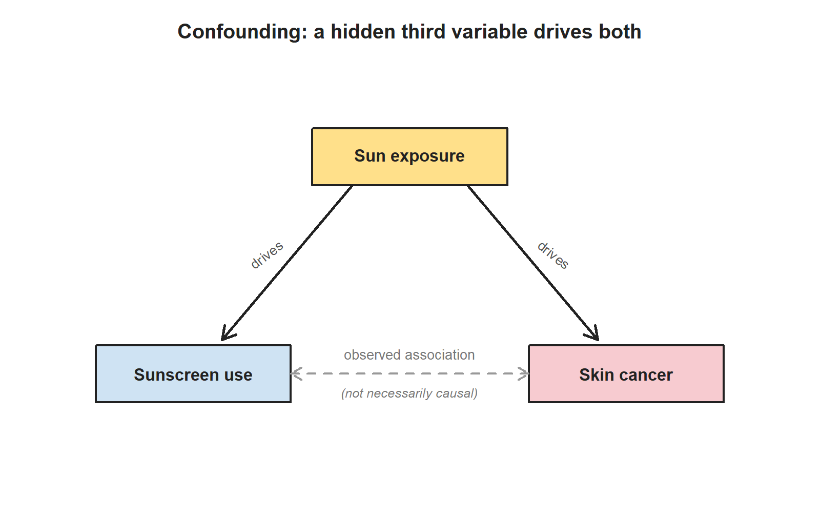
Diagram: sun exposure points to both sunscreen use and skin cancer; sunscreen use and skin cancer are joined by a dashed observed-association arrow labeled not necessarily causal. — Sun exposure drives both sunscreen use and skin cancer, so the two are associated even though neither causes the other.

This is why a careful observational study can show association but cannot, on its own, prove causation. A confounder might always be hiding. Random assignment — which only experiments can do — is what breaks that bind.

A handful of other words that come up in this conversation:

Anecdotal evidence: drawing a conclusion from one or two striking cases (“my uncle smoked his whole life and lived to 95, so smoking must not be that bad”). Striking and memorable; not evidence. But: an anecdote can be a useful starting point that motivates a real study. In 1958, a Vancouver general practitioner noticed that several of his elderly patients with a specific heart-valve condition were also experiencing severe gastrointestinal bleeding. That observation prompted the research that eventually identified Heyde Syndrome. Anecdote alone wasn’t proof; it was a useful question.
Overclaiming. Going beyond what the data support — usually by saying “X causes Y” when the data only support “X is associated with Y.” It is one of the most common reading errors in popular science writing.

Example: reading a study design

In Week 1 we met an observational study of air pollution and preterm birth: researchers collected California hospital records for 143,196 births and computed each pregnancy’s average exposure to several pollutants. Higher PM₁₀ exposure was associated with higher preterm-birth rates.

Reading the design this week:

Type of study? Observational. Nobody assigned anyone to a level of pollution exposure.
Population the study is really about? Births in Southern California in 1989–1993, or some closely-related population. Whether the results generalize to other places (rural areas, different decades, different pollution mixes) is a separate judgment.
Causal claim? Not directly. The association is real, but many confounders are possible — maternal income, neighborhood resources, occupational exposures, prenatal care access. The observational design cannot rule them out by itself.
Useful? Absolutely. The association is striking enough to motivate further studies, regulatory questions, and follow-up research with better confounder control.

Now compare to the Week 1 LEAP trial: same Week 1 study, very different design.

Type of study? Randomized experiment.
Population? Infants at risk of peanut allergy.
Causal claim? Defensible. Random assignment, large sample, pre-registered outcome.
Caveats? Still: one study, one population, one specific protocol. The general lesson — “introduce peanut early, not late” — does not automatically apply to children without the enrollment-criteria risk factors.

Both studies are useful evidence. Neither is the final word on anything. That is the Week 2 habit we want.

Common mistakes

These come up every Week 2 quarter.

“A random sample is a perfect sample.” No. A random sample removes one specific kind of bias (the bias of who you chose). It does not protect you from non-response, coverage gaps, or small sample size.
“Every experiment is a clinical trial.” Most aren’t. A classroom soda-preference experiment, a study assigning students to different study materials, a study assigning chick embryos to different supplemented diets — all experiments.
“Random assignment proves the treatment caused the outcome.” It strongly supports a causal claim. It does not prove one. Sample size, adherence, dropout, and replication all still matter.
“Anecdotes are useless.” Not quite. Anecdotes are useless as evidence and useful as questions.
“Observational means biased; experimental means clean.” Observational studies can be carefully designed and still produce real, useful evidence. Experiments can have their own problems (sham surgery, blinding failures, ethical limits on what you can randomize). The two designs do different jobs.
“Confounder = anything that affects the outcome.” No — a confounder must be associated with both the explanatory variable and the response variable. (Sun exposure is associated with both sunscreen use and skin cancer. That’s what makes it a confounder.)

What you should be able to do by Friday

By the end of Week 2 you should be able to:

Identify the population and the sample in a short study description, and judge whether the sample is likely to be representative.
Distinguish a population parameter from a sample statistic.
Name common sources of sample bias (convenience, voluntary response, non-response) and recognize each when you read about one.
Decide whether a study is observational or experimental.
Decide whether causal claims from a given study are defensible.
Name a plausible confounding variable when an observational study reports an association.
Recognize blind / placebo / double-blind designs in human studies and explain why they matter.

Homework 1 covers Week 1 + Week 2 material together. It is handled separately (see below).

Assignments this week

📄 Monday exit ticket — observational vs experimental snap check, plus a parameter-vs-statistic check. Aim for 3–5 minutes.
Download the Monday exit ticket (PDF)
📄 Wednesday exit ticket — scope-of-inference work on two studies from Week 1, one observational and one experimental. Aim for 8–12 minutes.
Download the Wednesday exit ticket (PDF)
🔒 Friday quiz — handled through Blackboard or in class as directed. The quiz prompt is not posted here. Exact timing and submission details live in Blackboard.
🔒 Homework 1 (biweekly, Weeks 1–2) — posted and submitted through Blackboard. Due near the start of Week 3; exact due date is on Blackboard.

Reuse

CC BY-SA 3.0.