Week 10 — Probability as risk and diagnosis

MATH 21003 · Introduction to Statistical Methods · Fall 2026 · Week 10 (Oct 26–30, 2026)

Why this week matters

A great deal of health and policy reasoning comes down to a single word: risk. What is the chance this test result is wrong? Given a positive screening result, what is the chance the patient actually has the disease? These are probability questions, and answering them well is the difference between a calm clinic and a panicked one.

This week treats probability as risk — a long-run chance — and then puts it to work on diagnostic testing. The skills are not new so much as renamed. In Week 5 you read conditional proportions off a two-way table (“among the smokers, what fraction…”). This week that becomes conditional probability (“among the people who tested positive, what is the chance…”). The Week 2 habit of asking where did these numbers come from, and for what population is what makes the week’s punchline — base rates matter — land.

The rhythm: Monday introduces probability-as-risk and conditional probability. Wednesday practices the diagnostic table — sensitivity, specificity, and completing a two-way table. Friday’s quiz works a full screening-test case: false positives, false negatives, and what a positive result really means when the disease is rare.

Probability as long-run risk

A probability is a number between 0 and 1 that describes how often something happens in the long run. If a condition has a probability of \(0.093\) in some population, that means: among many, many people from that population, about \(9.3\) out of every \(100\) have it. Probability is the long-run proportion — exactly the kind of proportion you have been reading off tables since Week 3, now read as a chance.

Two small pieces of vocabulary make the rest of the week easier. A probability of \(0\) means the event never happens; a probability of \(1\) means it always happens; everything real lives in between. And the complement rule: the chance an event does not happen is one minus the chance it does. If the chance a test comes back positive is \(0.07\), then the chance it comes back negative is \(1 - 0.07 = 0.93\). That is the entire arithmetic of complements, and it is worth saying out loud because so much diagnostic reasoning is just “the positives and the negatives have to add to everyone.”

When we say a screening test carries a “\(7\%\) false-positive risk,” we are making a long-run statement: out of many healthy people tested, about \(7\) in \(100\) will get a positive result anyway. Holding that long-run reading in mind is what keeps the rest of the week honest.

Conditional probability: the chance within a subgroup

Most useful risks are conditional — they describe the chance of something within a particular subgroup. We write the conditional probability of \(A\) given \(B\) as \(P(A \mid B)\), read “the probability of \(A\), among those for whom \(B\) is true.” It is computed exactly like a Week 5 conditional proportion: restrict to the subgroup \(B\), then ask what fraction of that subgroup has \(A\).

The ISLBS textbook tabulates a large population by age group and diabetes status (counts in thousands):

A two-way table with age groups in rows (under 20, 20 to 44, 45 to 64, 65 and over, and a total row) and columns for Diabetes, No diabetes, and Total, with counts in thousands. The 45 to 64 row is shaded. Beneath the table are two shaded boxes. The left box computes the probability of diabetes given age 45 to 64 as 13,400 divided by 81,926, about 0.164. The right box computes the probability of age 45 to 64 given diabetes as 13,400 divided by 29,100, about 0.461. — A two-way table of a U.S. population by age group and diabetes status, counts in thousands, with row totals. The under-20, 20-44, 45-64, and 65-and-over rows show diabetes and no-diabetes counts; the 45-64 row is highlighted. A total row reads 29,100 with diabetes and 284,220 without, out of 313,320. Below the table, two boxes contrast P(diabetes given 45-64) = 13,400 / 81,926 which is about 0.164, against P(45-64 given diabetes) = 13,400 / 29,100 which is about 0.461 — the same two numbers answering different questions.

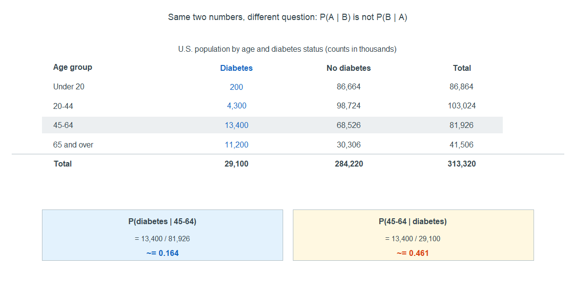
Overall, the chance a randomly chosen person has diabetes is \(29{,}100 / 313{,}320 \approx 0.093\). But among people 65 and over, the chance is \(11{,}200 / 41{,}506 \approx 0.27\) — about three times higher. That second number is a conditional probability: restrict to the 65-and-over subgroup, then take the fraction with diabetes. Conditioning on a subgroup can move a risk a lot, which is why “the overall rate” and “the rate among older adults” are genuinely different statements.

The trap: \(P(A \mid B)\) is not \(P(B \mid A)\)

Here is the single most important idea of the week, and the one most often gotten wrong. The two directions of a conditional probability are different numbers. “The chance of diabetes given you are 45–64” is not the same as “the chance you are 45–64 given that you have diabetes,” even though both use the same cell count.

Read both off the table. Of the \(81{,}926\) thousand people aged 45–64, \(13{,}400\) have diabetes, so

\[P(\text{diabetes} \mid \text{45–64}) = \frac{13{,}400}{81{,}926} \approx 0.164.\]

But of the \(29{,}100\) thousand people with diabetes, \(13{,}400\) are aged 45–64, so

\[P(\text{45–64} \mid \text{diabetes}) = \frac{13{,}400}{29{,}100} \approx 0.461.\]

Same numerator, different denominators, very different answers — \(16\%\) versus \(46\%\). The question “given which group?” decides which denominator you use. Flipping the condition flips the denominator, and that is why the two numbers come apart.

This is not a curiosity. It is the diagnostic-testing problem in disguise. A test’s advertised accuracy is usually a statement like “the chance of a positive result given the disease.” What a patient actually wants to know is the reverse: “the chance of the disease given a positive result.” Those are \(P(A \mid B)\) and \(P(B \mid A)\), and the rest of the week is about why they can be wildly different.

Diagnostic tests: sensitivity and specificity

A diagnostic test sorts people two ways — they either have the condition or not, and the test reads either positive or negative. That is a two-by-two table, and two conditional probabilities describe how good the test is:

Sensitivity = \(P(\text{test} + \mid \text{disease})\) — among people who have the disease, the chance the test catches it. The complement is the false-negative rate.
Specificity = \(P(\text{test} - \mid \text{no disease})\) — among people who are healthy, the chance the test correctly clears them. The complement is the false-positive rate.

For the mammogram example ISLBS uses, sensitivity is \(0.89\) (so the false-negative rate is \(11\%\)) and specificity is \(0.93\) (so the false-positive rate is \(7\%\)). Read those as conditional probabilities in the “given disease status” direction: given a woman has breast cancer, there is an \(89\%\) chance the mammogram is positive; given she does not, there is a \(7\%\) chance it is positive anyway. Both are statements about the test, conditioned on the truth.

Notice the direction. Sensitivity and specificity condition on what is true and ask what the test says. The patient’s question runs the other way — it conditions on what the test says and asks what is true. To answer it we need one more ingredient.

What a positive test really tells you: predictive values and base rates

The number a patient actually wants is the positive predictive value (PPV): \(P(\text{disease} \mid \text{test} +)\) — among everyone who tests positive, the fraction who truly have the disease. Its partner is the negative predictive value (NPV): \(P(\text{no disease} \mid \text{test} -)\). These run in the patient’s direction, and — this is the heart of the week — they depend on how common the disease is to begin with, the base rate (also called prevalence).

The cleanest way to see it is to run a hypothetical population through the test. Imagine \(100{,}000\) women screened, with a breast-cancer prevalence of \(0.35\%\):

A two-panel diagnostic figure. The left panel is a tree starting from 100,000 screened, splitting into breast cancer 350 and no cancer 99,650, and then each splitting into test-positive and test-negative branches: 311.5 true positives and 38.5 false negatives among those with cancer, and 6,975.5 false positives and 92,674.5 true negatives among those without. The right panel is a two-by-two table of the same four counts, with a callout that positive tests total 7,287 and the positive predictive value is 311.5 divided by 7,287, about 4 percent. — A diagram following 100,000 screened women through a tree and into a two-by-two table. Of 100,000, about 350 have breast cancer and 99,650 do not. Among the 350 with cancer, the 89%-sensitive test gives about 311.5 true positives and 38.5 false negatives. Among the 99,650 without cancer, the 7% false-positive rate gives about 6,975.5 false positives and 92,674.5 true negatives. The total number of positive tests is 311.5 plus 6,975.5 equals 7,287, and the positive predictive value is 311.5 divided by 7,287, about 4 percent.

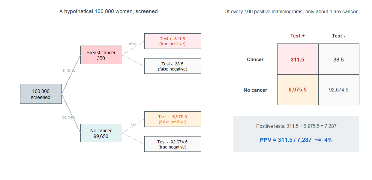
Walk it through. Of \(100{,}000\) women, about \(350\) have cancer and \(99{,}650\) do not. The test catches \(89\%\) of the \(350\) — about \(311.5\) true positives — and misses the rest. But it also flags \(7\%\) of the \(99{,}650\) healthy women — about \(6{,}975.5\) false positives. So the total number of positive results is \(311.5 + 6{,}975.5 = 7{,}287\), and of those, only \(311.5\) truly have cancer:

\[\text{PPV} = \frac{311.5}{7{,}287} \approx 0.04.\]

Read that out loud: of every 100 women with a positive mammogram, only about 4 actually have breast cancer. The test is good — \(89\%\) sensitive — and yet a positive result is probably a false alarm. Nothing is wrong with the test. The disease is simply rare, so the small percentage of false positives among the many healthy women outnumbers the true positives among the few sick ones. This is the \(P(A \mid B)\)-versus-\(P(B \mid A)\) trap with stakes: sensitivity (\(89\%\)) and PPV (\(4\%\)) point in opposite emotional directions.

The base rate is the lever. Hold the test fixed and ask how PPV changes as the disease becomes more common:

A rising curve on axes where the horizontal axis is prevalence as a percent from 0 to 30 and the vertical axis is positive predictive value as a percent from 0 to 100. The curve climbs steeply at first and then flattens. A red point near a prevalence of 0.35 percent sits at a PPV of about 4 percent, labeled mammogram screening. A green point at 10 percent prevalence sits at a PPV of about 59 percent. — A curve of positive predictive value against prevalence, for a fixed test with sensitivity 89% and specificity 93%. The curve rises steeply from near zero and then levels off. The mammogram point at a prevalence of 0.35% sits near a PPV of about 4%; a second point at 10% prevalence sits near a PPV of about 59%. The figure is labeled an instructor-built schematic.

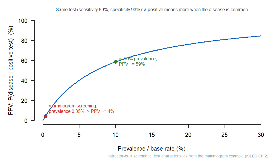
Same test, different worlds. At a \(0.35\%\) base rate the PPV is about \(4\%\); at a \(10\%\) base rate the very same test has a PPV near \(59\%\). A positive result means much more when the disease is common — for instance, when a test is run on people already showing symptoms rather than on the whole population. This is also why even a near-perfect test struggles against a very rare condition: a prenatal cfDNA screen with \(98\%\) sensitivity and \(99.5\%\) specificity, applied at a prevalence of \(1\) in \(800\), still yields a PPV of only about \(20\%\). Rarity is hard to beat.

The honest clinical reading, then, is never “the test is \(93\%\) accurate, so a positive means I’m \(93\%\) likely to be sick.” The right reading runs the patient’s direction and remembers the base rate: given this positive result, and given how common the disease is in people like me, what is the chance I actually have it? Often a positive screen is a reason for a second, better test — not a diagnosis.

Common mistakes

“Sensitivity is the chance I’m sick given a positive test.” No — that is PPV. Sensitivity conditions on being sick and asks what the test says; PPV conditions on the positive test and asks what’s true. Different directions, often very different numbers.
“A \(93\%\)-accurate test means a positive is \(93\%\) likely to be right.” Not when the disease is rare. The mammogram is \(89\%\) sensitive and a positive is only about \(4\%\) likely to be cancer.
“Base rate doesn’t matter if the test is good.” It always matters. The same test gives PPV \(\approx 4\%\) at a \(0.35\%\) base rate and \(\approx 59\%\) at a \(10\%\) base rate.
“\(P(A \mid B)\) equals \(P(B \mid A)\).” Almost never. Same cell, different denominators: \(P(\text{diabetes}\mid\text{45–64})\approx 0.16\) but \(P(\text{45–64}\mid\text{diabetes})\approx 0.46\).
“A false positive means the test is broken.” No — false positives are a built-in, expected fraction of healthy people (here, \(7\%\)). A good test still produces them.
“A negative result means I definitely don’t have it.” Not quite — the false-negative rate is the chance a truly sick person tests negative. NPV, not certainty, is the honest reading.

What you should be able to do by Friday

By the end of Week 10 you should be able to:

read a probability as a long-run risk, and use the complement rule (\(P(\text{not } A) = 1 - P(A)\));
compute a conditional probability \(P(A \mid B)\) from a two-way table by restricting to the subgroup;
explain, with a table, why \(P(A \mid B)\) and \(P(B \mid A)\) are different, and identify which one a question is asking for;
define sensitivity and specificity as conditional probabilities, and name their false-negative and false-positive complements;
build a hypothetical-population table from a prevalence, a sensitivity, and a specificity, and read PPV and NPV off it;
explain why a positive test can still be probably wrong when the disease is rare — the base-rate effect.

Assignments this week

Monday check. A short concept check on reading a probability as a risk and a conditional probability from a small table. Aim for about 3–5 minutes in class. Sheet: Week 10 Monday exit ticket.
Wednesday check. A short application completing a diagnostic two-way table and reading sensitivity, specificity, and a conditional probability. Aim for about 8–12 minutes in class. Sheet: Week 10 Wednesday exit ticket.
🔒 Friday quiz — handled through Blackboard or in class as directed. The quiz prompt is not posted here. Exact timing and submission details live in Blackboard.
🔒 Homework 5 (biweekly, Weeks 9–10) — posted and submitted through Blackboard. It spans last week and this one; due near the start of Week 11.

Reuse

CC BY-SA 3.0.