Week 1 — Data, evidence, and statistics

MATH 21003 · Introduction to Statistical Methods · Fall 2026 · Week 1 (Aug 24–28, 2026)

Why this week matters

Statistics is not a stack of formulas. It is a way to evaluate evidence — to decide what you can and cannot reasonably claim from a set of numbers. Before any technique works, you have to be able to look at a dataset and answer four basic questions:

Who or what is being measured?
What was measured about them?
What is the question we’re trying to answer?
What does the data, on its face, show?

This week is about getting fluent at those four questions on a small scale. By Friday you will look at a short study description and a small table and be able to talk back to it in clear, careful sentences. The bigger questions — how the data were collected, what biases could be hiding inside it, what claims it does and does not support — start in earnest in Week 2.

What counts as data?

When researchers measure or record something, they usually organize the result as a dataset: a structured collection of observations, recorded in a consistent way, so anyone reading the dataset later can see what was measured, on whom, and how.

Two small examples we will keep coming back to this semester.

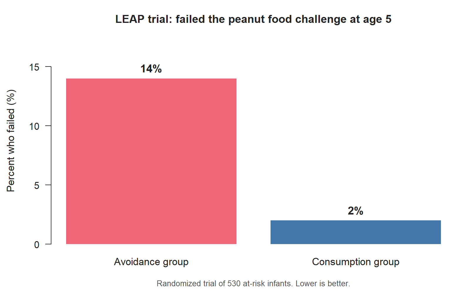
The LEAP trial. A public-health team studies whether early peanut exposure helps prevent peanut allergies in young children. They enroll 530 infants who are at risk of developing peanut allergy, randomly assign each child to either eat peanut products regularly (the “consumption” group) or avoid them (the “avoidance” group), and check at age five whether each child can safely eat peanuts. The final dataset records, for each child, which group they were in and whether they passed the food challenge. The reported result is striking: about 14% of children in the avoidance group failed the food challenge, compared with about 2% in the consumption group.

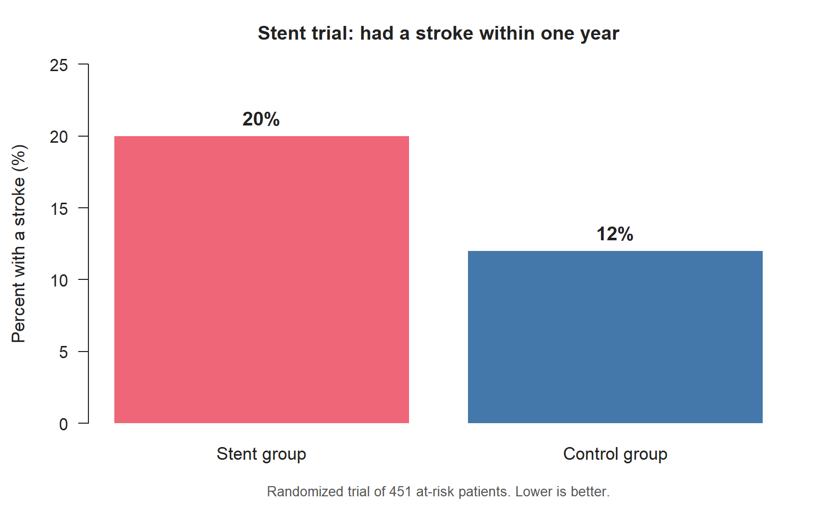
Bar chart comparing a 14 percent failure rate in the avoidance group to a 2 percent failure rate in the consumption group. — About 14% of the avoidance group failed the food challenge, versus about 2% of the consumption group — the gap that motivated introducing peanut early.

The stent trial. A different team runs a randomized study of 451 patients at risk of stroke. Patients in the treatment group receive a stent (a small mesh tube placed in a narrow artery) plus standard medical management; patients in the control group receive the standard medical management alone. The dataset records, for each patient, which group they were in and whether they had a stroke within 30 days and within one year. The reported result is also striking — but in the opposite direction: about 20% of patients in the stent group had a stroke within a year, compared with about 12% of patients in the control group.

Bar chart comparing a 20 percent stroke rate in the stent group to a 12 percent stroke rate in the control group. — About 20% of the stent group had a stroke within a year, versus about 12% of the control group — a striking result pointing the opposite way from LEAP.

Two well-run randomized studies; two striking results that point in opposite directions. The point isn’t that one is right and one is wrong. The point is that statistics is what lets you read each dataset carefully enough to decide what it does and does not support. We will return to both studies more than once this semester.

The key point right now: the dataset is what makes the analysis possible. Statistics starts when you can read the dataset.

Cases, variables, and data tables

Most datasets you see in this class will look like a table — rows and columns:

Patient ID	Treatment group	Passed food challenge?
100522	Peanut consumption	Yes
103358	Peanut consumption	Yes
105069	Peanut avoidance	Yes
994047	Peanut avoidance	Yes
997608	Peanut consumption	Yes

The vocabulary:

A case is one row. In this table each case is one child in the study.
A variable is one column. Here the variables are patient ID, treatment group, and passed food challenge?.
A data table (or data matrix) is the whole grid.

Cases are not always people. Here are some examples of cases you’ll see this term:

One patient on a hospital ward.
One breath sample from an asthma study.
One birth in a hospital records database.
One county in a public-health comparison.
One frog egg clutch in a biology study of maternal investment.

Whenever you read a new study description, the first thing to ask is: what is one case here? If you can answer that, the rest of the dataset’s structure usually clicks into place.

Sometimes a data table contains a blank, missing entry, or a code like NA. That usually means the value was not recorded for that case. It is not a new variable; it is a missing value for an existing variable.

Types of variables

Once you know what your cases are, the next question is what kind of variables they have. There are two main types.

Numerical variables

A numerical variable records a number where the numerical relationships are meaningful — you can sensibly add, subtract, average, or compare two values.

Continuous numerical variables can take any value within a range. Height in centimeters, systolic blood pressure in mmHg, PM₁₀ pollution levels in micrograms per cubic meter — all continuous.
Discrete numerical variables jump between separate values, usually integers. Number of hospital admissions per day, age in whole years — discrete.

A telephone number is not a numerical variable, even though it looks like digits. You can’t sensibly average phone numbers.

Categorical variables

A categorical variable records a label that tells you which group the case belongs to. The possible labels are called the levels of the variable.

A nominal categorical variable has levels with no natural ordering. Race, sex, dining station, blood type — nominal.
An ordinal categorical variable has levels that do have a natural order. Pain rating on a 0–10 scale grouped into “low / moderate / severe”, or age grouped into 5-year bins — ordinal.

Some variables look numerical but are best treated as categorical in context. If a researcher records data from 11 specific study sites and labels them 1 through 11, the site number is technically a number but it doesn’t make sense to “average two sites.” In context, the site label is categorical.

Response and explanatory variables

When a study asks a question like “does this affect that,” the “that” is the response variable (the outcome of interest) and the “this” is the explanatory variable (the variable the study is examining to see how the response changes).

Three quick examples:

Research question	Explanatory variable	Response variable
Does early peanut exposure reduce peanut-allergy rates?	Treatment group (consumption vs avoidance)	Passed the food challenge at age 5? (yes / no)
Does PM₁₀ exposure during pregnancy increase the chance of preterm birth?	Average gestational PM₁₀ exposure	Preterm-birth status (yes / no)
Does altitude affect frog reproductive investment?	Altitude of the study site	Clutch size, egg size, clutch volume

Two important habits:

“Response” and “explanatory” are properties of the research question, not of the variables themselves. The same variable could be a response in one study and an explanatory variable in another.
Not every variable in a dataset has a role. In the frog example, the researchers also recorded latitude and body size of the mother. Latitude is environmental context; body size is an auxiliary variable. Neither is the explanatory or the response variable of this study.

When you read a study description, identify the research question first, then point at which variables fill which role.

Evidence, claims, and context

A dataset, by itself, is just rows and columns. It becomes evidence when someone uses it to support a claim — and that claim is only as good as the dataset behind it.

Three habits to start practicing this week:

Read the numbers in context. A two-way table that shows ~14% of children in the LEAP avoidance group failed the food challenge and ~2% in the consumption group failed it is striking. So is a summary that shows 20% of stent-group patients had a stroke versus 12% of control-group patients. Each number tells you a lot, but no single number tells you everything. (We’ll ask “could the difference be due to chance?” in Week 11, and “what about other studies?” in Week 14.)
Distinguish what was measured from what wasn’t. If a study collected age, sex, and blood pressure but didn’t collect exercise habits, you cannot say anything about exercise from that dataset.
Be honest about how strong a single study’s evidence is. One study, even a well-run one, is one study. The LEAP and stent trials together illustrate this in opposite directions. We will get a lot more careful about this in Weeks 2, 11, and 14.

This isn’t about being cynical. It is about being honest.

Example: reading a small study dataset

Suppose a research team studies whether a shallow-breathing technique helps reduce asthma symptoms. They enroll 600 adults aged 18–69 who already rely on medication, randomly split them into two groups (one practicing the technique, one not), and at the end of the study score each participant on a 0–10 scale for symptom severity, medication use, activity level, and overall quality of life.

Use the four habits from the last section:

What is one case? One adult asthma patient enrolled in the study.
What variables were recorded? Group assignment (technique vs not), and four 0–10 scores (symptom severity, medication use, activity, quality of life).
Which variables are categorical? Numerical? Group is categorical (nominal). The four scores are numerical — you could argue they are discrete because they are whole numbers on a 0–10 scale, or treat them as continuous because they are summary scores of underlying quantities. Either is defensible if you say which one you mean.
What is the response, and what is the explanatory variable? Each of the four scores can be a response variable; group assignment is the explanatory variable.

That’s the kind of reading we want by Friday.

Common mistakes

These tend to come up in Week 1 and are worth heading off now.

“Case = patient.” Not always. A case might be a birth, a county, a clutch of eggs, or a day of measurements. Read the dataset description carefully before assuming.
“Numerical-looking = numerical variable.” Year, zip code, study site number, patient ID — all “look numerical” but they don’t necessarily mean anything as a number. In context they are often categorical labels.
“This variable IS the response variable.” Response and explanatory roles depend on the question being asked, not on the variable itself.
“The numbers speak for themselves.” They don’t. Numbers without a description of how they were collected, who they came from, and what was not measured are nearly impossible to read honestly.
“One striking result settles the question.” A single study can be a strong start but is rarely the end of the story. We’ll develop this throughout the term.

What you should be able to do by Friday

By the end of Week 1 you should be able to:

Read a short study description and identify what one case is.
Identify the variables in the dataset and classify each as numerical (continuous or discrete) or categorical (nominal or ordinal).
State the research question and identify the response and explanatory variables.
Recognize when a variable is auxiliary — neither the response nor the explanatory variable of the study in question.
Read a small data matrix (5–10 rows) and a small two-way summary table without panic.
Write one or two careful sentences about what a small dataset does and does not show.

The Wednesday in-class exit ticket is about this. The Friday quiz and Homework 1 are too — they are handled separately (see below).

Assignments this week

📄 Monday exit ticket — short concept check on the LEAP and stent variable types. Aim for 3–5 minutes.
Download the Monday exit ticket (PDF)
📄 Wednesday exit ticket — read two small datasets (MCU films and a frog data matrix) and classify the variables. Aim for 8–12 minutes.
Download the Wednesday exit ticket (PDF)
🔒 Friday quiz — handled through Blackboard or in class as directed. The quiz prompt is not posted here. Exact timing and submission details live in Blackboard.
🔒 Homework 1 (biweekly, covers Weeks 1–2) — posted and submitted through Blackboard. Due near the start of Week 3; exact due date is on Blackboard.

Reuse

CC BY-SA 3.0.