Week 15 — Comparative inference synthesis and the bridge onward
Where this week starts
Fifteen weeks ago this course made a promise: that a statistical procedure is a decision rule with assumptions and operating characteristics, not a mechanical route to a p-value. Every week since has kept half of it by building a family of procedures and calibrating it. This week keeps the other half. You push one question, one data set, and one estimand through five of the routes this course built — an exact procedure, a large-sample likelihood procedure, a resampling procedure, a rank-based procedure, and a Bayesian decision — and then read the five results side by side.
Week 14 closed the theoretical circle by putting Bayes rules, admissibility, and minimaxity back into the decision-theoretic frame of Week 1; what it left unfinished is the practical consequence. You now own five machines that can be pointed at the same two-group comparison, and nothing so far has said what to do when they return different verdicts. That is the ordinary situation, not the exotic one.
What makes the comparison tractable is to stop asking which procedure is right and ask three narrower questions of each in turn. What quantity does it estimate? What has to be true for its stated calibration to hold? And at the sample size in front of me, does that calibration hold, or is it a limit statement wearing a finite-sample costume? Separating those turns most apparent contradictions into a map of the assumptions your conclusion rests on, and by the end “the procedures disagree” should read as an unfinished sentence rather than a result.
Why this matters beyond the theorem
Here is the stake in its most common form. A laboratory runs a small randomized comparison, gets a two-sided p-value of \(0.059\) from a \(t\) test, and reports no significant difference. A colleague reruns the same data as a likelihood-ratio test against the chi-square reference, gets \(0.034\), and reports a significant improvement. A third computes a posterior probability of \(0.965\) that the new material is better and recommends adoption. All three are correct arithmetic on the same twelve observations; what differs is the reference distribution and, in the third case, what the number is a probability of.
The failure mode is not miscomputation. It is that whoever writes the report picks the number suiting the conclusion and never states which calibration was chosen or why. That choice, made after seeing all three, is the selective-inference error of Week 9 operating on whole procedures rather than individual hypotheses, and it is invisible in the finished report.
What you will be able to do
- Construct exact, large-sample likelihood, permutation, rank-based, and Bayesian procedures for one target on the same data, stating each one’s conditions before applying it.
- Identify the estimand each route targets, and say when two routes reporting similar numbers are nonetheless estimating different quantities.
- Compute the exact finite-sample size of an asymptotically calibrated test where that is available, and rank the routes by how well calibrated they are at the sample size in hand.
- Diagnose a material disagreement by attributing it to a specific broken condition rather than to procedural preference.
- Write a comparative conclusion stating the estimand, the calibration claim, the stress test, and what the result does not support.
Terms and notation worth fixing
| Symbol or term | Meaning as used in this course |
|---|---|
| \(\Delta = \mu_A - \mu_B\) | this unit’s estimand: the difference in mean response between two coatings |
| estimand | the population quantity a procedure targets, fixed before any procedure is chosen |
| calibration claim | the operating characteristic asserted: exact level, limiting level, coverage, or posterior probability |
| \(\Lambda\), \(2 \log \Lambda\) | here \(\Lambda\) is the likelihood ratio itself, so the statistic on the chi-square scale is \(2 \log \Lambda = 2\{\ell(\hat\theta) - \ell(\hat\theta_0)\}\). Week 5 names that same chi-square-scale statistic \(\Lambda\), so read across the two pages by the formula, not the letter |
| \(W_A\) | the Wilcoxon rank-sum statistic: the sum of the pooled ranks falling in group \(A\) |
| sharp null | the Week 10 hypothesis that each unit’s response is identical under either treatment |
| \(L(\theta, a)\), \(R(\theta, \delta)\) | loss and risk, exactly as in Weeks 1 and 14 |
Two conventions hold throughout. “Route” means a procedure together with the reference distribution it is calibrated against, so the \(t\) statistic referred to \(t_{10}\) and the same information referred to \(\chi^2_1\) are two routes, not one. Every interval quoted is a two-sided nominal \(95\) per cent interval and every p-value is two-sided.
One estimand, five inferential routes
Fix the target before fixing the machinery. Twelve nominally identical aluminium coupons are randomly assigned, six to a reformulated coating \(A\) and six to the incumbent coating \(B\), and each is pulled to failure on the same rig. The recorded adhesion strengths, in coded units, are
\[A: 47, 56, 59, 61, 64, 67 \qquad \text{and} \qquad B: 42, 46, 52, 53, 55, 58 .\]
These numbers are illustrative, but the assignment mechanism is part of the setup: the coupons were randomized, and that licenses one of the five routes outright. The estimand is \(\Delta = \mu_A - \mu_B\), the difference in mean adhesion over the population this batch represents. Three routes target this \(\Delta\), one targets something related but different, and one returns a posterior for it. Skip this step and you are comparing numbers that are not comparable.
What each route is actually estimating
The exact route models the twelve values as independent draws from \(N(\mu_A, \sigma^2)\) and \(N(\mu_B, \sigma^2)\) with a common unknown \(\sigma^2\), and uses the pivot \(T = (\bar{X}_A - \bar{X}_B - \Delta) / (S_p \sqrt{1/n_A + 1/n_B})\), whose distribution is exactly \(t_{10}\) for every \((\mu_A, \mu_B, \sigma)\). That parameter-free distribution is Week 4’s pivotal quantity, and inverting it gives the interval.
The large-sample likelihood route keeps the model and the data and changes the reference. \(2 \log \Lambda\) compares the maximized log-likelihood over the full model with its maximum under \(\Delta = 0\), and Wilks’ theorem sends it to \(\chi^2_1\) provided the model is correct, the null value is an interior point of the parameter space, the log-likelihood is twice differentiable with non-singular information there, and the models differ by exactly one free parameter. All four hold here — and none mentions \(n = 12\).
The permutation route drops the normal model. Under the sharp null of Week 10 — coupon \(i\) fails at the same load under either coating — the responses are fixed and only the assignment is random, so each of the \(\binom{12}{6} = 924\) splits was equally likely. Its validity comes from the design, and its null is strictly stronger than “the means are equal”.
The rank route replaces the values by their pooled ranks and uses \(W_A\). Provided the response is continuous, so that ties have probability zero, its null distribution is the same whatever that distribution is — which is all “distribution-free” means. A test statistic has no influence function; the functional the test inverts to does. That functional is the Hodges-Lehmann one, the median of all \(n_A n_B\) pairwise differences \(A_i - B_j\), and its influence function is bounded. Attach Week 12’s distinction to that fact rather than reading it as Week 13’s robustness: Week 12 called rank procedures resistant, since they bound the influence of a wild value by discarding the information in every value and changing the estimand to do it, whereas the M-estimators of Week 13 bound influence while holding the target roughly where it was. So the Hodges-Lehmann functional estimates a shift, but only under a shift model. When the shapes differ it estimates an exceedance probability, and quoting that as a statement about means is the Week 12 error.
The Bayesian route treats \(\Delta\) as random, puts a prior on it, and returns a posterior and then a decision. Its output is not an interval with a repeated-sampling coverage claim; it is a probability statement conditional on the data, the model, and the prior.
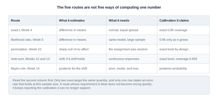
Where each calibration comes from and what it promises
Read that table by its last two columns, because that is where the routes separate. Only the exact route claims coverage holding at \(n = 12\); the likelihood route claims a level only in the limit; the permutation and rank routes are exact at any \(n\) but only for their own nulls; and the Bayesian route claims no repeated-sampling property unless you compute one.
In the normal two-sample model you can check this exactly. Writing \(\mathrm{RSS}_1\) for the within-group sum of squares and \(\mathrm{RSS}_0\) for the sum of squares about the grand mean, profiling \(\sigma^2\) out of the likelihood gives
\[2 \log \Lambda = n \log \frac{\mathrm{RSS}_0}{\mathrm{RSS}_1} = n \log\!\left(1 + \frac{t^2}{n - 2}\right),\]
using \(\mathrm{RSS}_0 = \mathrm{RSS}_1 + \frac{n_A n_B}{n} (\bar{x}_A - \bar{x}_B)^2\). So \(2 \log \Lambda\) is a strictly increasing function of \(t^2\): the two routes order the sample space identically and can differ only through their cutoffs. Setting \(2 \log \Lambda \ge 3.841\), the chi-square \(0.95\) quantile on one degree of freedom, gives \(\lvert t \rvert \ge 1.942\) at \(n = 12\), against the exact cutoff \(2.228\). Since \(T\) is exactly \(t_{10}\) under the null, each asymptotic cutoff \(c\) has a true size \(P(\lvert T_{10} \rvert \ge c)\) that can be computed rather than guessed:
| Route and cutoff | Rejects when | Exact size at \(n = 12\) |
|---|---|---|
| Wald, \(\chi^2_1\) at \(3.841\) | \(\lvert t \rvert \ge 1.789\) | \(0.104\) |
| likelihood ratio, \(\chi^2_1\) at \(3.841\) | \(\lvert t \rvert \ge 1.942\) | \(0.081\) |
| score, \(\chi^2_1\) at \(3.841\) | \(\lvert t \rvert \ge 2.170\) | \(0.055\) |
| exact \(t\), \(t_{10}\) at \(2.228\) | \(\lvert t \rvert \ge 2.228\) | \(0.050\) |
The ordering \(\text{Wald} \ge 2 \log \Lambda \ge \text{score}\) holds in this instance, as it did in Week 5’s example, and here it becomes an ordering of actual error rates. Week 5 was explicit that no theorem guarantees that ordering, so it is a fact about these twelve coupons rather than a rule. A test with nominal level \(0.05\) and actual size \(0.104\) is not a \(0.05\) test; it is a \(0.104\) test with a misleading label. That is the most useful thing to know before reading a disagreement between an exact route and an asymptotic one at small \(n\).
Reading a disagreement rather than resolving it
When two routes give different verdicts, the reflex is to decide which one is correct. Resist it long enough to classify the disagreement first, because the three kinds have different consequences for what you write down.
A hierarchy of questions when procedures conflict
Ask them in this order. Are the routes estimating the same quantity? If one reports a mean difference and another a Hodges-Lehmann shift, they can differ without either being wrong, and under asymmetry they differ systematically — Week 13’s exponential example had the mean and the median a factor of \(1.44\) apart. Nothing is reconciled by argument here; you must choose which functional the question is about.
If the estimand is shared, is one calibration failing at this sample size? The table above settles that in the normal two-sample model: the asymptotic routes are anti-conservative at \(n = 12\), so their smaller p-values are partly an artefact of calibration rather than evidence. Where no closed form is available, Week 7’s size study supplies the same information by simulation.
If the estimands agree and the calibrations hold, is one route’s condition simply false? A permutation test on observational data inherits nothing from a randomization that never happened, and a Wald interval near a boundary behaves differently on two scales — which is why Week 5 insisted the likelihood-ratio statistic is invariant to reparameterization and the Wald statistic is not. Only when all three questions come back clean is the disagreement genuine, and then it is almost always small. Marginal evidence is a finding; disguising it by shopping for a reference is what this course exists to make impossible.
Worked example — five routes through one two-group adhesion trial
Carry all five routes on the twelve coupons through to a number; every figure below comes from those twelve integers.
Step 1: the common summaries. The group means are \(\bar{x}_A = 59\) and \(\bar{x}_B = 51\), so \(\hat\Delta = 8.0\). The within-group sums of squares are \(246\) and \(176\), so \(\mathrm{RSS}_1 = 422\), \(s_p^2 = 422/10 = 42.2\) and \(s_p = 6.496\). The standard error of the difference is \(s_p \sqrt{1/6 + 1/6} = 6.496 \times 0.5774 = 3.751\).
Step 2: the exact route. Here \(t = 8.0 / 3.751 = 2.133\) on \(10\) degrees of freedom, a two-sided p-value of \(0.059\). Inverting the pivot with \(t_{10, 0.975} = 2.228\) gives \(8.0 \pm 2.228 \times 3.751\), that is \((-0.36, 16.36)\). The interval covers zero, so at level \(0.05\) this route does not reject.
Step 3: the large-sample likelihood route. The grand mean is \(55\) and \(\mathrm{RSS}_0 = 614\); equivalently \(614 = 422 + 3 \times 8^2\) from the identity above. Then \(2 \log \Lambda = 12 \log(614/422) = 4.500\) and \(P(\chi^2_1 \ge 4.500) = 0.034\), so this route rejects. Inverting the same statistic with \(\mathrm{RSS}(\Delta_0) = 422 + 3(8 - \Delta_0)^2\), the acceptance set \(12 \log\{1 + 3(8 - \Delta_0)^2 / 422\} \le 3.841\) reduces to \((8 - \Delta_0)^2 \le 53.07\) and gives \((0.71, 15.29)\). The Wald and score statistics, \(n(\mathrm{RSS}_0 - \mathrm{RSS}_1)/\mathrm{RSS}_1\) and \(n(\mathrm{RSS}_0 - \mathrm{RSS}_1)/\mathrm{RSS}_0\), come to \(5.460\) and \(3.752\), with nominal p-values \(0.019\) and \(0.053\) — three asymptotically equivalent statistics spread across the decision boundary.
Step 4: the resampling route. Under the sharp null, enumerate all \(924\) splits of the twelve observed values into groups of six and compute each difference in means. Exactly \(58\) give an absolute difference of at least \(8.0\), so the exact permutation p-value is \(58/924 = 0.063\); inverting the same test over candidate shifts gives \((-0.50, 16.33)\). Note what the test did not assume: no normality, no equal variances, no large sample. The interval asks for more. Inverting a permutation test over shifts means testing a family of sharp nulls with a stated constant effect, in Week 10’s words, so it presumes the coating adds the same \(\Delta\) to every coupon — an assumption the randomization does not supply, and the same one the rank route needs for its shift model.
Step 5: the rank route. In the pooled ordering, group \(A\) occupies ranks \(3, 7, 9, 10, 11, 12\), so \(W_A = 52\). Its null distribution is that of a sum of six ranks drawn without replacement from \(1\) through \(12\); \(19\) of the \(924\) subsets sum to at least \(52\), and that distribution is symmetric about its mean \(39\), so the exact two-sided p-value is \(38/924 = 0.041\). The Hodges-Lehmann estimate, the median of the \(36\) pairwise differences \(A_i - B_j\), is \(8.5\), and the shifts this test does not reject run from the sixth smallest to the sixth largest of those differences, giving \((1, 17)\) with exact coverage \(1 - 38/924 = 0.959\) rather than \(0.950\) — Week 4’s discreteness conservatism.
Step 6: the Bayesian route. Hold \(\sigma\) at \(s_p = 6.496\) and put a sceptical conjugate prior \(\Delta \sim N(0, \tau^2)\) with \(\tau = 6\) on the difference, chosen because past reformulations of this coating have moved mean adhesion by less than about \(12\) coded units, which \(\tau = 6\) places at two prior standard deviations. Writing \(\sigma_{\hat\Delta} = 3.751\) for the standard error of \(\hat\Delta\), Week 14’s calculation gives a normal posterior with mean \(w \hat\Delta\) and variance \(\tau^2 \sigma_{\hat\Delta}^2 / (\tau^2 + \sigma_{\hat\Delta}^2)\), where the shrinkage weight is \(w = \tau^2 / (\tau^2 + \sigma_{\hat\Delta}^2) = 36 / (36 + 14.07) = 0.719\). So the posterior is \(N(5.75, 3.18^2)\), with \(P(\Delta > 0 \mid x) = 0.965\), \(P(\Delta > 5 \mid x) = 0.594\), and central \(95\) per cent credible interval \((-0.48, 11.99)\).
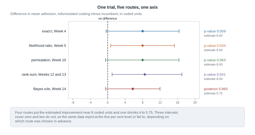
Step 7: the decision, stated as a decision. Suppose the smallest improvement worth requalifying the line for is \(\Delta_0 = 5\) coded units, with actions adopt and retain. Taking the loss to be \(c_1\) for adopting when \(\Delta \le 5\), \(c_2\) for retaining when \(\Delta > 5\), and zero otherwise, the Bayes rule adopts exactly when \(P(\Delta > 5 \mid x) \ge c_1 / (c_1 + c_2)\). With equal costs the threshold is \(1/2\) and the posterior probability \(0.594\) says adopt, narrowly; if a wrong adoption costs three times a missed improvement the threshold rises to \(0.75\) and the same posterior says retain. The loss is doing visible work — Week 1’s lesson in its final form.
What this licenses: an improvement of about \(8\) coded units, with compatible values running roughly from zero to sixteen, and evidence at the boundary of conventional significance in every well-calibrated route. What it does not license: quoting \(0.034\) without saying its reference has actual size \(0.081\) here; reading \(0.965\) as a p-value or an error rate; or treating the five intervals as five estimates of one number, since one estimates a shift and one is a posterior summary.
The same reasoning, transferred
Run the same questions on a binary response. A second trial randomizes twenty coupons, ten per coating, and records whether each passes a peel test: \(8\) of \(10\) pass under \(A\) and \(3\) of \(10\) under \(B\), so \(\Delta = p_A - p_B\) and \(\hat\Delta = 0.50\). Conditioning on the eleven total passes, the exact route is Fisher’s exact test, whose reference is the hypergeometric distribution over tables with these margins; summing the probabilities of all tables at least as unlikely as the observed one gives a two-sided p-value of \(0.070\). The likelihood route computes \(G^2 = 2 \sum O \log(O/E) = 5.300\) against \(\chi^2_1\), giving \(0.021\). With independent uniform priors the posteriors are \(\mathrm{Beta}(9, 3)\) and \(\mathrm{Beta}(4, 8)\), and \(P(p_A > p_B \mid x) = 0.985\).
What stayed the same is the shape of the finding: the exact route is markedly more conservative than the asymptotic one, and the posterior probability is a third kind of number. What changed is instructive. The permutation route adds no fifth column, because under complete randomization the permutation distribution of the passes in group \(A\) is the hypergeometric — exact and resampling coincide rather than merely agree. The rank route collapses too, since with two values the ranks carry what the counts carry. Five routes became three, for reasons in the response rather than the analyst’s preference.
Second worked example — the same trial with one heavy-tailed reading
Now stress-test the comparison. Suppose the weakest coupon in group \(A\) had failed at \(35\) rather than \(47\) — possible when the substrate carries a microscopic flaw, and exactly the kind of tail a normal model does not have. Nothing else changes, so group \(A\) reads \(35, 56, 59, 61, 64, 67\).
Step 1: what moves in the summaries. Now \(\bar{x}_A = 57\) and \(\hat\Delta = 6.0\), while the within-group sum of squares in \(A\) rises from \(246\) to \(654\), giving \(\mathrm{RSS}_1 = 830\), \(s_p = 9.110\), and a standard error of \(5.260\). The estimate fell by a quarter and its standard error grew by two fifths, so \(t = 6.0 / 5.260 = 1.141\) with a two-sided p-value of \(0.281\), and the interval widens to \((-5.72, 17.72)\).
Step 2: the routes built on the magnitudes follow it down. With \(\mathrm{RSS}_0 = 938\), \(2 \log \Lambda = 12 \log(938/830) = 1.468\) with p-value \(0.226\) and inverted interval \((-4.22, 16.22)\). The permutation test now finds \(268\) of the \(924\) splits at least as extreme, a p-value of \(0.290\). The posterior becomes \(N(3.39, 3.96^2)\), so \(P(\Delta > 0 \mid x) = 0.804\) and \(P(\Delta > 5 \mid x) = 0.342\): under equal costs the Bayes rule now says retain where it said adopt.
Step 3: the route that reads only the ordering. The value \(35\) is still the smallest of the twelve, so group \(A\) occupies ranks \(1, 7, 9, 10, 11, 12\) and \(W_A = 50\) instead of \(52\), an exact two-sided p-value of \(86/924 = 0.093\) — the statistic moved two rank units while \(t\) fell by nearly half. The Hodges-Lehmann estimate is unchanged at exactly \(8.5\), because only the six differences involving that coupon moved, and they lay below the median both before and after, so the eighteenth and nineteenth ordered differences are the same \(8\) and \(9\) as before. The distribution-free interval does move, from \((1, 17)\) to \((-7, 17)\), since its lower endpoint is the sixth smallest pairwise difference and those six are now exactly the six smallest.
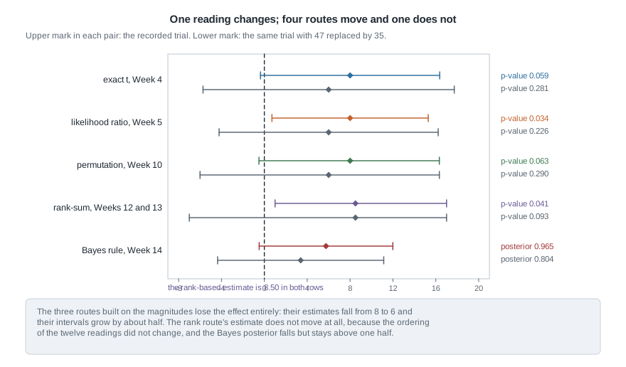
Step 4: which conclusion is defensible. Work the hierarchy. The estimands still differ — four routes target \(\Delta\) and the rank route a shift — so part of the gap between \(0.093\) and \(0.281\) is not a contradiction, and the calibrations hold or fail as before. What is new is that a normality assumption merely unverifiable at \(n = 12\) is now visibly implausible, and the routes leaning on magnitudes pay for it in variance. A permutation test is exact in level here and still loses power: exactness protects the error rate, not the sensitivity.
So the defensible report is not “the rank test found an effect”. It is that one coupon carries a large share of the evidence; that the mean-based routes see an improvement of \(6.0\) coded units with compatible values from about \(-6\) to \(17\); that a rank-based analysis, insensitive to how extreme that coupon is, still places the shift near \(8.5\) but no longer excludes zero; and that the experiment is too small to separate these readings. Refitting with a bounded influence function is Week 13’s repair and belongs beside the others, not instead of them. Note that the Bayesian route did not escape either: holding \(\sigma\) at \(s_p\) sent the inflated spread straight into the posterior, so robustness is a property of the model you wrote down, not of the philosophy you wrote it in.
The misreading to avoid
The sentence to dismantle ends most comparative studies: “the five procedures disagree, so we report the one that is most appropriate for these data.” In practice “most appropriate” means “chosen after seeing all five”, a data-dependent selection with no correction attached. Whatever guarantee the selected route carried described a procedure fixed in advance; select it after the fact and the guarantee is gone, exactly as in Week 9, and the loss is invisible in the output. The repair is procedural: name the primary route and its conditions before computing, and present the others as sensitivity analyses allowed to disagree.
A second misreading treats the Bayesian number as a stronger version of the frequentist one: “\(P(\Delta > 0 \mid x) = 0.965\), so the p-value of \(0.059\) was too conservative.” They address different questions. The posterior probability is conditional on the data, the model, the fixed \(\sigma\), and a prior; the p-value describes how a procedure behaves across repetitions under the null. The near-coincidence is instructive rather than reassuring: under a flat reference prior on \((\mu_A, \mu_B, \log \sigma)\) the posterior for \(\Delta\) is exactly \(8.0 + 3.751 \, T_{10}\), so the credible interval is numerically identical to \((-0.36, 16.36)\) while asserting something about that particular interval which the \(t\) interval never asserts. Week 4’s warning that coverage is a property of the procedure, not of a realized interval, keeps them apart.
A third misreading generalizes from the stress test: “the rank route was stable, so rank methods are always safer.” Its estimate was stable; its interval moved by eight coded units, its achieved coverage is \(0.959\) rather than \(0.950\), its estimand is a shift only under a shift model, and at an exactly normal model it needs about one extra observation in twenty to match the \(t\) procedure. And agreement does not validate either: five routes sharing a data set, a design, and in three cases a model will often agree, which rules out arithmetic error and little else.
The bridge to the graduate sequence
This course completes the common inferential spine, and the syllabus records which later course picks up which thread. Read the map as a claim about vocabulary rather than content: what you carry forward is the habit of naming an estimand, stating a calibration, and pricing an assumption.
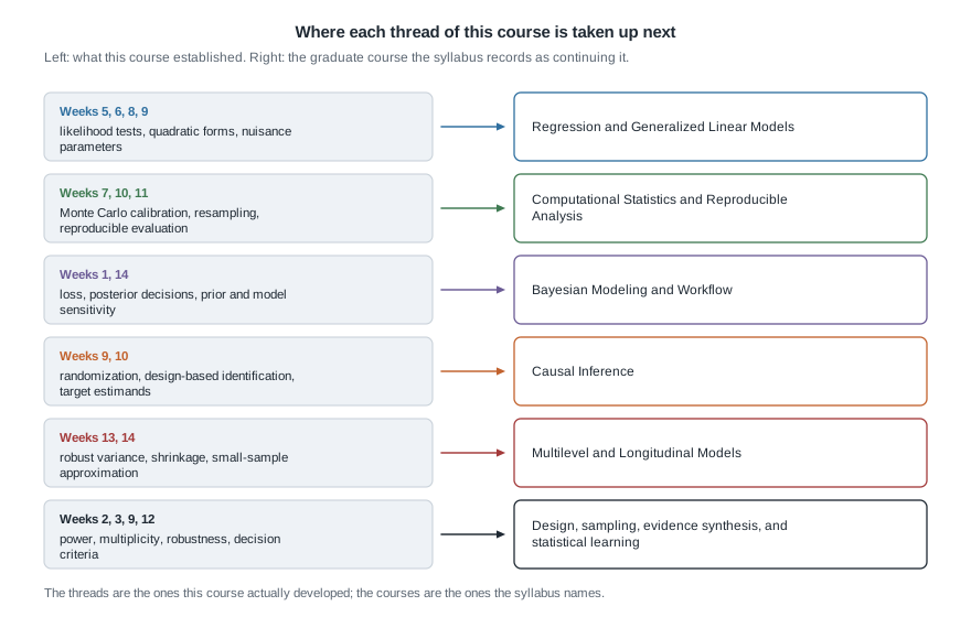
Graduate Regression and Generalized Linear Models takes the likelihood tests, quadratic forms, and nuisance parameters of Weeks 5 through 9, and Computational Statistics and Reproducible Analysis the Monte Carlo calibration and resampling of Weeks 7, 10, and 11. Bayesian Modeling and Workflow takes the loss and posterior decisions of Weeks 1 and 14, with the computation this course left alone, while Causal Inference takes randomization, design-based identification, and target estimands. Multilevel and Longitudinal Models take robust variance and shrinkage; design, sampling, evidence synthesis, and statistical learning take power, multiplicity, and decision criteria under selection.
Reporting a comparison honestly
The portfolio artifact this course asks for states a target, a procedure, a calibration claim, an assumption, a stress test, and a corrected conclusion. The checklist below is that requirement as six sentences you can work through, and the first line is the one most reports omit.
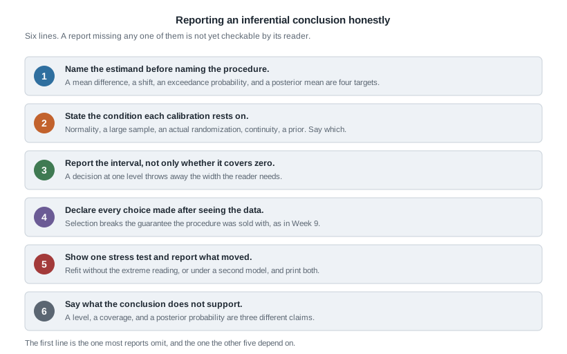
Applied to the adhesion trial, a passing report reads like this. The estimand is the difference in mean adhesion; the primary route, fixed in advance, is the exact two-sample procedure, giving \(8.0\) coded units with interval \((-0.36, 16.36)\) and a two-sided p-value of \(0.059\) under normality with a common variance. The permutation, rank-based, and likelihood-ratio analyses follow as declared sensitivity analyses, the last noted as coming from a reference whose actual size here is \(0.081\). One extreme coupon moves every mean-based conclusion. The evidence supports a provisional improvement near \(8\) coded units, not a demonstrated superiority.
a <- c(47, 56, 59, 61, 64, 67)
b <- c(42, 46, 52, 53, 55, 58)

t.test(a, b, var.equal = TRUE)                    # exact route
wilcox.test(a, b, conf.int = TRUE)                # rank route

lr_stat <- function(a, b) {
  n    <- length(a) + length(b)
  rss1 <- sum((a - mean(a))^2) + sum((b - mean(b))^2)
  rss0 <- sum((c(a, b) - mean(c(a, b)))^2)
  n * log(rss0 / rss1)
}
pchisq(lr_stat(a, b), df = 1, lower.tail = FALSE) # large-sample route

pooled <- c(a, b)
splits <- combn(12, 6)
gaps   <- apply(splits, 2, function(i) mean(pooled[i]) - mean(pooled[-i]))
mean(abs(gaps) >= abs(mean(a) - mean(b)))         # permutation route

tau <- 6
se  <- sqrt((sum((a - mean(a))^2) + sum((b - mean(b))^2)) / 10 / 3)
pnorm(5, tau^2 / (tau^2 + se^2) * (mean(a) - mean(b)),
      sqrt(tau^2 * se^2 / (tau^2 + se^2)), lower.tail = FALSE)
Practice on your own
- Verify \(\mathrm{RSS}_0 = \mathrm{RSS}_1 + \frac{n_A n_B}{n} (\bar{x}_A - \bar{x}_B)^2\) for two groups of unequal size, then use it to show \(2 \log \Lambda\) is strictly increasing in \(t^2\). Explain why that makes the two routes’ p-values differ while their orderings of the sample space agree.
- Reproduce the exact-size column of the calibration table by simulation at \(n_A = n_B = 6\) and again at \(n_A = n_B = 30\), with a Monte Carlo standard error on each figure. At what sample size does the Wald route’s size first fall below \(0.06\)?
- Construct a two-group data set on which the permutation and \(t\) tests give materially different p-values, and diagnose which feature caused the gap. Then construct a second on which the rank-sum test rejects and the \(t\) test does not, with no observation extreme.
- Change the design rather than the data: suppose the coupons were drawn from two production lines already running the two coatings rather than randomized. Which routes remain valid, which lose their justification, and what would the estimand become?
- Redo the Bayesian route with \(\tau = 2\) and \(\tau = 20\), and plot \(P(\Delta > 5 \mid x)\) against \(\tau\). Identify the \(\tau\) at which the equal-cost decision flips, and say what you would need to know about past reformulations to defend either side of it.
Where to read more
- For the theory tying these routes together at graduate depth, see MIT OpenCourseWare 18.655 Mathematical Statistics, where the regularity conditions of Wilks’ theorem are written out in full.
- For secondary treatments of the procedures compared here — the \(t\) procedure, the likelihood-ratio test, rank methods, resampling, and Bayesian inference — see Penn State STAT 415.
- The optional Hogg, McKean, and Craig alignment for this week is Chapters 4 through 11, taken as synthesis rather than as new reading. The book is optional and never required for this course; availability and licence terms for every source listed here remain unconfirmed.
- Everything on this page runs in base R and
stats: The R Project for Statistical Computing and Quarto. - Course pages: the notes overview, the syllabus, the schedule, and the resources page.
Where this goes next
There is no Week 16. What follows is the rest of the graduate sequence, and the thread you carry into it is narrower than any single procedure: name the estimand, state the calibration and the condition it rests on, price the assumption by moving it, and say what the conclusion does not support. Every course on the map above will ask for that sentence in its own vocabulary.
If a strand of this comparison felt thin, the unit that built it is the place to return to rather than this one: Week 4 for the duality that makes an interval out of a test family, Week 5 for why three asymptotically equivalent statistics disagree at \(n = 12\), Week 10 for the design-based validity of the permutation route, Week 12 for what the rank-sum statistic estimates, and Week 14 for the posterior expected loss that turned a probability into a decision. Use the notes overview to see the sixteen units in order and the schedule for the weekly rhythm this page belongs to.