Week 14 — Bayes rules, admissibility, minimaxity, and shrinkage
Where this week starts
Week 1 built the frame this course stands on. A procedure \(\delta\) carries data to an action, a loss \(L(\theta, a)\) prices the mistake, and the risk \(R(\theta, \delta) = E_\theta L(\theta, \delta(X))\) records the performance at each possible truth. It also left a hole. Risk is a function of \(\theta\), two risk functions usually cross, and “which procedure is better” means nothing until you say how a whole curve is compressed into one number worth minimizing. Every week since dodged that by fixing a side condition first: hold the size and maximize power, hold coverage and minimize width. This week asks the question directly.
There are two natural compressions. Average the curve against a prior \(\pi\) on \(\Theta\) and you get the Bayes risk \(r(\pi, \delta)\), whose minimizer is a Bayes rule. Take the worst point, \(\sup_\theta R(\theta, \delta)\), and its minimizer is a minimax rule. Beside them sits a third notion needing no number: \(\delta\) is inadmissible when some rule has risk no larger at every \(\theta\) and strictly smaller at one. Admissibility is the weakest demand and the hinge for the other two, because Bayes rules are nearly always admissible and admissible rules nearly always Bayes.
By the end of the week you should move in both directions: from a posterior and a loss to the Bayes action, and then out of the Bayesian frame to that same rule’s frequentist risk as a function of \(\theta\), which says where it beats the usual unbiased estimator and where it loses. Every model here is conjugate, so the decision theory stays in view; posterior computation and modelling workflow belong to a separate course.
Why this matters beyond the theorem
A calibration laboratory holds ten instruments and estimates each instrument’s offset from its own measurements, independently. Reporting ten separate sample means is the obvious procedure, unbiased and efficient coordinate by coordinate. If what the laboratory cares about is the total squared error across all ten offsets, that procedure is inadmissible: whatever the ten true offsets are, a rule pulling all ten estimates toward a common centre has strictly smaller expected total squared error. No assumption was violated and no reading was bad. The loss was total while the procedure was coordinatewise, and nothing in the ten standard errors discloses the gap.
The mirror image is the prior. A Bayes rule built from a confident prior looks superb on the single number it was designed to minimize and can still be far worse than the sample mean over the stretch of the parameter space where the prior was wrong. Bayes risk cannot show that, because averaging is what it does. The risk function can.
What you will be able to do
- Derive a Bayes rule by minimizing posterior expected loss, stating the conditions under which that pointwise minimization solves the Bayes-risk problem.
- Identify the Bayes action under squared-error, absolute-error, and zero-one loss, and say which moment or quantile each needs.
- Compute the frequentist risk of a Bayes rule exactly in a conjugate model, and locate where it beats the unbiased alternative and where it loses.
- Prove that a unique Bayes rule with finite Bayes risk is admissible, and that a constant-risk Bayes rule is minimax with a least favourable prior.
- Construct the prior making a binomial estimation problem hardest, and verify the constant risk.
- State the Stein phenomenon with its actual conditions, read a shrinkage factor as an estimated Bayes weight, and say what it does not claim.
Terms and notation worth fixing
| Symbol or term | Meaning as used in this course |
|---|---|
| \(\pi\), \(\pi(\theta \mid x)\) | a prior distribution on the parameter space \(\Theta\), and the posterior after observing \(x\) |
| \(\rho(\pi, a \mid x)\) | posterior expected loss, \(\int L(\theta, a) \, \pi(\theta \mid x) \, d\theta\): one number for one action at one data set |
| \(r(\pi, \delta)\) | Bayes risk, \(\int R(\theta, \delta) \, \pi(d\theta)\): the risk curve averaged against the prior |
| \(\delta_\pi\), \(r(\pi)\) | a Bayes rule, meaning any procedure minimizing \(r(\pi, \cdot)\), and the minimum value \(r(\pi) = \inf_\delta r(\pi, \delta)\) |
| \(\sup_\theta R(\theta, \delta)\) | maximum risk: the worst single point of a risk curve |
| admissible | no \(\delta'\) has \(R(\theta, \delta') \le R(\theta, \delta)\) for every \(\theta\) with strict inequality somewhere |
| least favourable | a prior \(\pi\) with \(r(\pi) \ge r(\pi')\) for every competing prior \(\pi'\) |
| \(\lVert a - \theta \rVert^2\) | total squared-error loss in \(p\) dimensions, \(\sum_{j=1}^{p} (a_j - \theta_j)^2\) |
Two conventions hold throughout. “Risk” unqualified always means frequentist risk, an expectation over the data at fixed \(\theta\), with no prior in it. And a Bayes rule is a rule, defined at every data set you might have seen rather than an estimate attached to the one you have, which is what makes it legitimate to ask for its risk function.
Bayes rules and the two summaries of risk
The Bayes criterion replaces an incomparable pair of curves with a comparable pair of numbers, at the cost of an input the frequentist frame does not supply. Once a prior is named the ordering is total, and the minimizer never has to be searched for across the space of rules.
Bayes risk and the exchange of integrals
Let the data have density \(f(x \mid \theta)\) and let \(\pi\) be proper, a genuine probability distribution on \(\Theta\). Write the Bayes risk out and exchange the order of integration:
\[r(\pi, \delta) = \int_\Theta \left[ \int_{\mathcal{X}} L\big(\theta, \delta(x)\big) f(x \mid \theta) \, dx \right] \pi(d\theta) = \int_{\mathcal{X}} \left[ \int_\Theta L\big(\theta, \delta(x)\big) \pi(\theta \mid x) \, d\theta \right] m(x) \, dx ,\]
where \(\mathcal{X}\) is the sample space, \(m(x) = \int f(x \mid \theta) \pi(d\theta)\) is the marginal density of the data, and \(\pi(\theta \mid x) = f(x \mid \theta) \pi(\theta) / m(x)\) is the posterior. The exchange is Tonelli’s theorem, needing only that the loss is nonnegative and jointly measurable.
Read the right-hand side. The inner bracket is the posterior expected loss \(\rho(\pi, \delta(x) \mid x)\), involving \(\delta\) only through the single value \(\delta(x)\), and the outer integral weights those brackets by \(m(x) \ge 0\). A rule therefore minimizes the whole integral as soon as it minimizes the bracket separately at each \(x\): writing \(\mathcal{A}\) for the action space, a Bayes rule is any \(\delta_\pi\) with
\[\delta_\pi(x) \in \arg\min_{a \in \mathcal{A}} \int_\Theta L(\theta, a) \, \pi(\theta \mid x) \, d\theta \qquad \text{for } m\text{-almost every } x .\]
Three conditions do work. The prior must be proper, so \(m(x)\) is finite and the posterior exists; with an improper prior the display has no right-hand side, and the rule computed from the formal posterior is called generalized Bayes, with no Bayes-risk optimality attached. A minimizer must exist for almost every \(x\), automatic when \(\mathcal{A}\) is compact and the posterior expected loss is continuous in \(a\). And some rule must have finite Bayes risk, or the comparison is vacuous.
The Bayes action under three losses
The recipe is mechanical, and the action changes with the loss although the posterior does not. Under squared-error loss \(L(\theta, a) = (\theta - a)^2\), expand about the posterior mean:
\[\rho(\pi, a \mid x) = E\big[(\theta - a)^2 \mid x\big] = \mathrm{Var}(\theta \mid x) + \big(E[\theta \mid x] - a\big)^2 ,\]
uniquely minimized at \(a = E[\theta \mid x]\) whenever the posterior second moment is finite. The Bayes action is the posterior mean and the minimum value is the posterior variance.
Under absolute-error loss \(L(\theta, a) = \lvert \theta - a \rvert\), take \(b > a\) and compare. On \(\{\theta \le a\}\) the loss rises by exactly \(b - a\); on \(\{\theta \ge b\}\) it falls by exactly \(b - a\); strictly between, it changes by \(a + b - 2\theta\), which lies between those extremes. Bounding the middle piece by its largest value gives
\[\rho(\pi, b \mid x) - \rho(\pi, a \mid x) \ \le \ (b - a) \big[ P(\theta < b \mid x) - P(\theta \ge b \mid x) \big] ,\]
so moving right strictly helps whenever less than half the posterior mass lies below \(b\), and the mirror-image bound says moving left helps whenever less than half lies above \(a\). The minimizer is therefore a posterior median. It needs \(E[\lvert \theta \rvert \mid x]\) finite, and need not be unique.
Under zero-one loss on a two-action testing problem, with \(\Theta_0\) and \(\Theta_1\) partitioning \(\Theta\) and unit loss for a wrong decision, the posterior expected loss of accepting is \(P(\theta \in \Theta_1 \mid x)\) and of rejecting is \(P(\theta \in \Theta_0 \mid x)\), so the Bayes rule picks the hypothesis with larger posterior probability. With costs \(c_{\mathrm{I}}\) for a false rejection and \(c_{\mathrm{II}}\) for a false acceptance it rejects when the posterior odds exceed \(c_{\mathrm{I}} / c_{\mathrm{II}}\). That threshold is a statement about consequences, not evidence, which is why a Bayes test carries no particular type I error rate.
For a symmetric unimodal posterior — the normal posterior of the first worked example — the posterior mean and median coincide, so squared-error and absolute-error loss select the same action. The zero-one loss just described belongs to a two-action testing problem and returns a hypothesis, not a point, so it is not in that comparison; its point-estimation counterpart is the limit of \(L(\theta, a) = \mathbf{1}\{\lvert \theta - a \rvert > \epsilon\}\) as \(\epsilon \downarrow 0\), whose Bayes action is a posterior mode and therefore agrees here as well. That agreement is a property of that posterior, not a general fact, which is why the loss looks invisible in the conjugate normal problem.
Where the argument needs care
Two cautions travel with it. Bayes risk is one number and hides the whole curve, which is why the rest of this page computes \(R(\theta, \delta_\pi)\) afterwards. And the construction depends on the prior, which at moderate sample sizes is no formality.
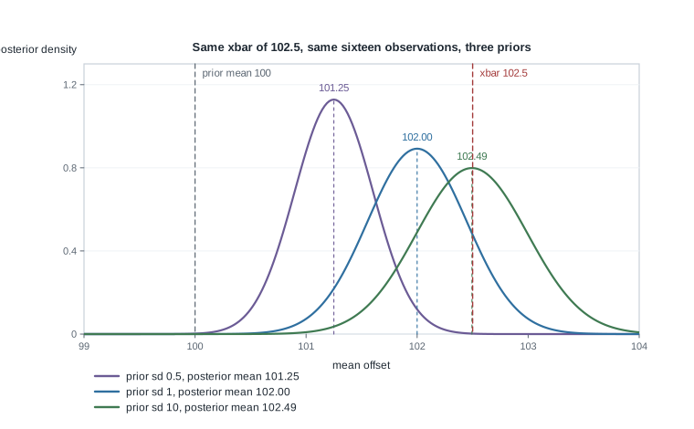
The figure uses the first worked example’s data: sixteen observations with sample mean \(102.5\) and known measurement standard deviation \(2\), so the standard error is \(0.5\). Holding the prior mean at \(100\) and moving only the prior standard deviation across \(0.5\), \(1\), and \(10\) shifts the posterior mean from \(101.25\) to \(102.00\) to \(102.49\). That spread of about \(1.25\) exceeds the half-width of any one of the three posteriors, so a reader told only the estimate cannot tell a strong data signal from a strong prior.
Admissibility, minimaxity, and least favourable priors
Admissibility asks nothing about averages or worst cases, only whether a rule is beaten outright everywhere at once. Few rules fail it, which makes it a minimal requirement rather than a criterion of choice: passing recommends nothing, since the rule that ignores the data and always reports the value \(7\) is admissible, no rule being able to beat it at \(\theta = 7\).
Bayes rules are almost always admissible
Proposition 1. If \(\delta_\pi\) is a Bayes rule for a proper prior \(\pi\), its Bayes risk \(r(\pi, \delta_\pi)\) is finite, and \(\delta_\pi\) is the unique Bayes rule up to sets of \(m\)-measure zero, then \(\delta_\pi\) is admissible.
Suppose some \(\delta\) dominates, so \(R(\theta, \delta) \le R(\theta, \delta_\pi)\) for all \(\theta\) with strict inequality somewhere. Averaging against \(\pi\) gives \(r(\pi, \delta) \le r(\pi, \delta_\pi)\), so \(\delta\) is itself Bayes; by uniqueness it agrees with \(\delta_\pi\) almost everywhere, hence has the same risk function, contradicting the strict inequality. Finiteness of \(r(\pi, \delta_\pi)\) keeps that comparison from reading \(\infty \le \infty\).
Proposition 2. If \(\Theta\) is an interval of the real line, \(R(\theta, \delta)\) is continuous in \(\theta\) for every rule considered, \(\pi\) assigns positive probability to every nonempty open subset of \(\Theta\), and \(r(\pi, \delta_\pi)\) is finite, then \(\delta_\pi\) is admissible even without uniqueness.
If \(\delta\) dominates with \(R(\theta_1, \delta) < R(\theta_1, \delta_\pi)\), continuity makes the strict inequality hold on an open interval around \(\theta_1\), which has positive prior probability, so \(r(\pi, \delta) < r(\pi, \delta_\pi)\) and \(\delta_\pi\) was not Bayes. Drop continuity and the improvement can hide at one point of prior probability zero; drop full support and it can hide outside the prior’s support.
The converse is a complete-class result, and its side conditions are part of the statement. For finite \(\Theta\), restrict attention to rules of finite risk. Their risk vectors, over all randomized rules, then form a convex subset \(S\) of \(\mathbb{R}^{\lvert \Theta \rvert}\) with finite entries, bounded below because the loss is nonnegative — randomizing averages risk vectors — and the admissible rules sit on its lower-left boundary. Suppose in addition that \(S\) is closed. Each such boundary point then carries a supporting hyperplane whose normal is nonzero; running the argument on the upward-closed set \(S + \mathbb{R}^{\lvert \Theta \rvert}_{+}\) forces the entries of that normal to be nonnegative, and a nonzero nonnegative vector has positive coordinate sum, so it can be rescaled to sum to one and read as a prior the rule is Bayes against. Closedness by itself is not enough: without a floor under the risks there need be no supporting hyperplane, and with the zero vector admitted as a normal there is nothing to rescale. For general \(\Theta\) no such statement holds unconditionally. Wald’s complete-class theorem assumes a compact \(\Theta\) on which \(R(\theta, \delta)\) is continuous for every rule considered, and even then the honest conclusion is that every admissible rule is generalized Bayes — minimizing formal posterior expected loss under a possibly improper prior — or a limit of Bayes rules. That last phrase is not a technicality: the estimator in the next section is such a limit and is inadmissible.
Constant risk, minimaxity, and the least favourable prior
A rule \(\delta^{*}\) is minimax when \(\sup_\theta R(\theta, \delta^{*}) = \inf_\delta \sup_\theta R(\theta, \delta)\). Searching all rules directly is hopeless, so the route goes through a prior.
Proposition 3. If \(\delta_\pi\) is a Bayes rule for a proper prior \(\pi\), \(r(\pi, \delta_\pi)\) is finite, and \(R(\theta, \delta_\pi) = c\) for every \(\theta\), then \(\delta_\pi\) is minimax and \(\pi\) is least favourable.
For any competing \(\delta\), a supremum is at least an average:
\[\sup_\theta R(\theta, \delta) \ \ge \ \int R(\theta, \delta) \, \pi(d\theta) = r(\pi, \delta) \ \ge \ r(\pi, \delta_\pi) = \int c \, \pi(d\theta) = c = \sup_\theta R(\theta, \delta_\pi) ,\]
the second inequality being only that \(\delta_\pi\) is Bayes for \(\pi\). Constancy is what turns the average on the right back into a supremum. For least favourability, any other prior \(\pi'\) has \(r(\pi') \le \int R(\theta, \delta_\pi) \pi'(d\theta) = c = r(\pi)\), since a minimum over rules is at most the value at \(\delta_\pi\). Constancy can be weakened: it suffices that \(\pi\) puts probability one on the set where \(R(\theta, \delta_\pi)\) attains its maximum.
Minimaxity inherits the weaknesses of worst cases. It optimizes against a configuration of \(\theta\) that may be implausible, and it does not imply admissibility: a minimax rule can be dominated by another minimax rule, which is exactly what happens next.
Shrinkage and the Stein phenomenon
Take \(X \sim N_p(\theta, \sigma^2 I_p)\) with \(\sigma^2\) known, under total squared-error loss \(L(\theta, a) = \lVert a - \theta \rVert^2\). The obvious rule \(\delta_0(X) = X\) has risk \(E_\theta \lVert X - \theta \rVert^2 = p \sigma^2\) at every \(\theta\), and it is minimax by a limiting version of Proposition 3: under the prior \(N_p(0, \tau^2 I_p)\) the minimum Bayes risk is \(p \sigma^2 \tau^2 / (\sigma^2 + \tau^2)\), which rises to \(p \sigma^2\) as \(\tau^2\) grows, so no rule can have maximum risk below \(p \sigma^2\). For \(p = 1\) and \(p = 2\) it is admissible as well. For \(p \ge 3\) it is not.
The James-Stein rule and its exact risk
The James-Stein rule pulls the whole vector toward the origin by a data-dependent factor:
\[\delta^{\mathrm{JS}}(X) = \left( 1 - \frac{(p - 2) \sigma^2}{\lVert X \rVert^2} \right) X .\]
An integration-by-parts identity for the normal density gives its risk in closed form,
\[R(\theta, \delta^{\mathrm{JS}}) = p \sigma^2 - (p - 2)^2 \sigma^4 \, E_\theta \!\left[ \frac{1}{\lVert X \rVert^2} \right] ,\]
and the subtracted term is strictly positive whenever \(p \ge 3\), so the risk lies strictly below \(p \sigma^2\) at every \(\theta\): domination is uniform, with no region where the sample vector wins. The condition \(p \ge 3\) enters twice, through \((p - 2)^2\) and because \(E_\theta \lVert X \rVert^{-2}\) is infinite for \(p \le 2\), where the display is not meaningful.
The expectation is exactly computable. Since \(\lVert X \rVert^2 / \sigma^2\) is noncentral chi-square with \(p\) degrees of freedom and noncentrality \(\lambda = \lVert \theta \rVert^2 / \sigma^2\), and that is a Poisson mixture of central chi-squares with \(p + 2K\) degrees of freedom for \(K \sim \mathrm{Poisson}(\lambda/2)\), the identity \(E[1 / \chi^2_m] = 1/(m - 2)\) gives \(E_\theta \lVert X \rVert^{-2} = \sigma^{-2} E[(p - 2 + 2K)^{-1}]\). At \(\theta = 0\), \(K = 0\) with probability one, so
\[R(0, \delta^{\mathrm{JS}}) = p \sigma^2 - (p - 2)^2 \sigma^4 \cdot \frac{1}{\sigma^2 (p - 2)} = 2 \sigma^2 ,\]
whatever \(p\) is. Jensen’s inequality on the convex map \(k \mapsto (p - 2 + 2k)^{-1}\), with \(E[2K] = \lambda\), bounds the risk above by \(p \sigma^2 - (p - 2)^2 \sigma^2 / (p - 2 + \lambda)\), so the guaranteed saving is at least \((p - 2)^2 \sigma^2 / (p - 2 + \lambda)\): it thins like \(1/\lambda\) as the true mean vector leaves the centre, and never reaches zero.
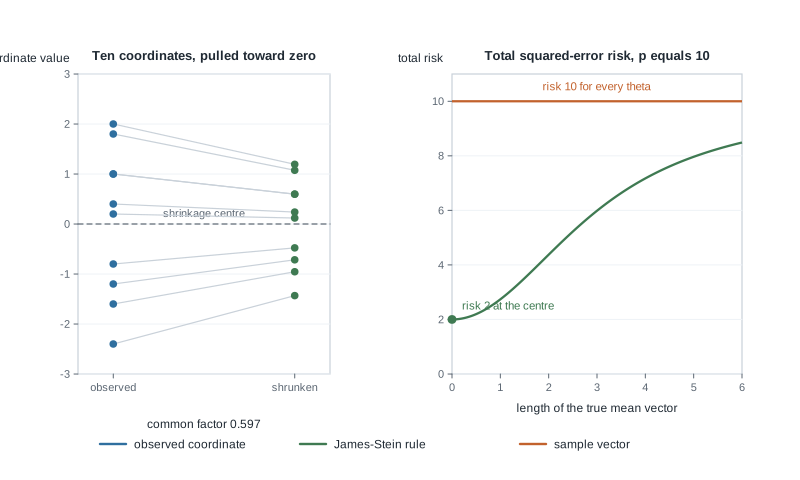
The left panel uses the observed vector \((2.0, -1.2, 0.4, 1.8, -0.8, 1.0, -2.4, 1.0, 0.2, -1.6)\) with \(\sigma^2 = 1\), whose squared length is \(19.84\), so the factor is \(1 - 8/19.84 = 37/62 \approx 0.597\) and every coordinate is multiplied by that one number: \(2.0\) becomes \(1.19\) and \(0.2\) becomes \(0.12\). The right panel plots the exact risk for \(p = 10\) and \(\sigma^2 = 1\): \(2.00\) at \(\lVert \theta \rVert = 0\) against the sample vector’s \(10\), about \(4.38\) at \(\lVert \theta \rVert = 2\), and about \(8.49\) at \(\lVert \theta \rVert = 6\), approaching \(10\) from below.
Shrinkage as an estimated Bayes weight
The factor is not a trick. Give the coordinates the exchangeable prior \(\theta_1, \dots, \theta_p\) independent \(N(0, \tau^2)\). Coordinatewise the posterior mean is the weighted average of the earlier section:
\[E[\theta_j \mid X] = \frac{\tau^2}{\tau^2 + \sigma^2} X_j = \left( 1 - \frac{\sigma^2}{\sigma^2 + \tau^2} \right) X_j ,\]
so the Bayes rule shrinks every coordinate by one common factor set by \(\tau^2\). Marginally the \(X_j\) are independent \(N(0, \sigma^2 + \tau^2)\), so \(\lVert X \rVert^2 / (\sigma^2 + \tau^2)\) is central chi-square with \(p\) degrees of freedom, and the same identity gives
\[E \!\left[ \frac{p - 2}{\lVert X \rVert^2} \right] = \frac{p - 2}{(\sigma^2 + \tau^2)(p - 2)} = \frac{1}{\sigma^2 + \tau^2} .\]
So in that marginal distribution \((p - 2) \sigma^2 / \lVert X \rVert^2\) is an unbiased estimator of the Bayes shrinkage weight \(\sigma^2 / (\sigma^2 + \tau^2)\), and the James-Stein rule is the conjugate Bayes rule with its one hyperparameter estimated from the same data. That is why the gain is largest near the origin, where the prior would have been right, and why it never becomes a loss: the risk identity holds at every \(\theta\), not merely on average under the prior.
Two limitations travel with it. The rule is itself inadmissible, since when \(\lVert X \rVert^2 < (p - 2) \sigma^2\) the factor is negative and the estimate points the wrong way; its positive-part version dominates it and is in turn inadmissible. And the centre is arbitrary: shrinking toward any fixed vector dominates just as well. Nothing requires the coordinates to be related, which is what makes the result feel paradoxical.
Worked example — the conjugate normal mean under squared-error loss
A reference standard is measured \(n = 16\) times on an instrument whose measurement standard deviation is known to be \(\sigma = 2\) coded units, so \(X_1, \dots, X_{16}\) are independent \(N(\theta, 4)\) and the sample mean is \(\bar{x} = 102.5\). Experience with instruments of this type is encoded as the conjugate prior \(\theta \sim N(\mu, \tau^2)\) with \(\mu = 100\) and \(\tau = 1\). The loss is squared error.
Step 1: the posterior. The likelihood depends on the data only through \(\bar{x}\), which is \(N(\theta, \sigma^2/n)\), so completing the square in the product of two normal densities gives a normal posterior whose precisions add:
\[\frac{1}{v_n} = \frac{n}{\sigma^2} + \frac{1}{\tau^2}, \qquad \mu_n = v_n \left( \frac{n \bar{x}}{\sigma^2} + \frac{\mu}{\tau^2} \right) .\]
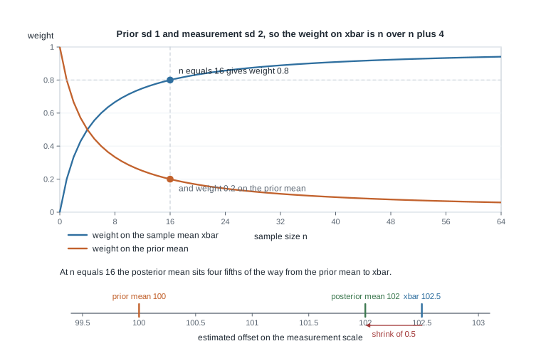
Write \(w = n \tau^2 / (n \tau^2 + \sigma^2)\). Multiplying numerator and denominator by \(\sigma^2 \tau^2\) turns the second display into \(\mu_n = w \bar{x} + (1 - w) \mu\) and the first into \(v_n = w \sigma^2 / n\). Here \(w = 16/20 = 0.8\), so \(\mu_n = 0.8 (102.5) + 0.2 (100) = 102.0\) and \(v_n = 0.8 \times 0.25 = 0.2\).
Step 2: the Bayes rule. The Bayes action is the posterior mean, so \(\delta_\pi(x) = w \bar{x} + (1 - w) \mu\): an explicit shrinkage of the sample mean toward the prior mean, by \(0.5\) units here. A \(95\) per cent posterior interval is \(102.0 \pm 1.96 \sqrt{0.2} = (101.12, 102.88)\), against the frequentist interval \(102.5 \pm 1.96 (0.5) = (101.52, 103.48)\).
Step 3: the frequentist risk, exactly. Forget the prior and treat \(\delta_\pi\) as a rule. The bias is \(w \theta + (1 - w) \mu - \theta = (1 - w)(\mu - \theta)\), so
\[R(\theta, \delta_\pi) = \mathrm{Var}_\theta\big(w \bar{X}\big) + \big(E_\theta \delta_\pi - \theta\big)^2 = w^2 \frac{\sigma^2}{n} + (1 - w)^2 (\theta - \mu)^2 ,\]
which is \(0.16 + 0.04 (\theta - 100)^2\) here, while \(R(\theta, \bar{X}) = \sigma^2/n = 0.25\) is flat.
Step 4: where each rule wins. The Bayes rule has smaller risk exactly when \((1 - w)^2 (\theta - \mu)^2 < (1 - w^2) \sigma^2 / n\). Divide by \((1 - w)^2\) and use \(1 - w = \sigma^2 / (n \tau^2 + \sigma^2)\), which turns \((\sigma^2/n)/(1 - w)\) into \(\tau^2 + \sigma^2/n\); the condition becomes \((\theta - \mu)^2 < (1 + w)(\tau^2 + \sigma^2/n)\). The right side is \(1.8 \times 1.25 = 2.25\), so the Bayes rule wins precisely for \(\lvert \theta - 100 \rvert < 1.5\) and loses outside, with unbounded risk far away.
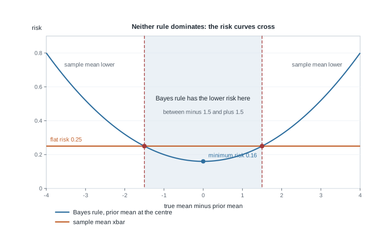
Step 5: the Bayes-risk scorecard. Averaging the risk curve against the prior and using \(E_\pi (\theta - \mu)^2 = \tau^2 = 1\) gives \(r(\pi, \delta_\pi) = 0.16 + 0.04 = 0.2\), agreeing with the posterior variance as it must, since that variance does not depend on the data. The sample mean scores \(r(\pi, \bar{X}) = 0.25\). On the prior’s own scorecard the Bayes rule wins by \(20\) per cent; on the risk function it loses over most of the real line.
What this licenses: an exact statement of the tradeoff, and — by Proposition 2, whose continuity and full-support conditions both hold — that \(\delta_\pi\) is admissible. What it does not license: that \(\delta_\pi\) is the better rule. Its maximum risk is infinite, so it is not minimax, and the data give no comfort about which \(\theta\) is in force: the observed \(\bar{x} = 102.5\) sits \(2.5\) units from the prior mean, so any \(\theta\) near it lies outside the interval \(\lvert \theta - 100 \rvert < 1.5\) on which \(\delta_\pi\) has the smaller risk.
The same reasoning, transferred
Run the identical argument on counts. Let \(X_1, \dots, X_n\) be independent Poisson with mean \(\theta\) under a conjugate Gamma prior with shape \(\alpha\) and rate \(\beta\). The posterior is Gamma with shape \(\alpha + \sum x_i\) and rate \(\beta + n\), and its mean is again a weighted average,
\[\frac{\alpha + \sum_i x_i}{\beta + n} = w \bar{x} + (1 - w) \frac{\alpha}{\beta}, \qquad w = \frac{n}{n + \beta} .\]
Take \(n = 20\), \(\alpha = 10\), \(\beta = 5\), so the prior mean is \(2\) and \(w = 0.8\), and suppose \(\sum x_i = 46\), so \(\bar{x} = 2.3\). The Bayes estimate is \(56/25 = 2.24\), which is \(0.8 (2.3) + 0.2 (2)\) as promised.
What stayed the same is the structure: conjugate prior, posterior mean as a weighted average, risk as variance plus squared bias, giving \(R(\theta, \delta_\pi) = w^2 \theta / n + (1 - w)^2 (\theta - \alpha/\beta)^2\). What changed is that the competitor’s risk is no longer flat, since \(\mathrm{Var}(\bar{X}) = \theta/n\) moves with \(\theta\). Here \(R(\theta, \delta_\pi) = 0.032 \theta + 0.04 (\theta - 2)^2\) against \(R(\theta, \bar{X}) = 0.05 \theta\), and equating them reduces to \(\theta^2 - 4.45 \theta + 4 = 0\) with roots \(1.25\) and \(3.2\). The Bayes rule wins on \((1.25, 3.2)\), an interval not symmetric about the prior mean \(2\): it leans toward large \(\theta\), where the sample mean is noisier and shrinkage buys more. Constant variance hid that asymmetry in the normal problem.
Second worked example — a minimax estimator for a binomial proportion
Let \(X \sim \mathrm{Binomial}(n, \theta)\) with \(n = 16\), under squared-error loss. The sample proportion \(X/n\) has risk \(\theta(1 - \theta)/n\): zero at the endpoints and largest in the middle, \(0.25/16 = 0.015625\) at \(\theta = 1/2\). That curve is far from flat, so Proposition 3 suggests hunting for a Bayes rule that flattens it.
Step 1: the Bayes rule for a beta prior. With \(\theta \sim \mathrm{Beta}(\alpha, \beta)\) the posterior is \(\mathrm{Beta}(\alpha + x, \beta + n - x)\), with mean \(\delta(x) = (x + \alpha)/M\) where \(M = n + \alpha + \beta\).
Step 2: its risk as a polynomial in \(\theta\). From \(E_\theta X = n\theta\) and \(\mathrm{Var}_\theta X = n\theta(1 - \theta)\), the bias is \((n\theta + \alpha)/M - \theta = \big(\alpha - (\alpha + \beta)\theta\big)/M\), so
\[M^2 R(\theta, \delta) = n \theta (1 - \theta) + \big(\alpha - (\alpha + \beta)\theta\big)^2 = \theta^2 \big[(\alpha + \beta)^2 - n\big] + \theta \big[n - 2\alpha(\alpha + \beta)\big] + \alpha^2 .\]
Step 3: force the risk constant. Both coefficients must vanish. The first gives \(\alpha + \beta = \sqrt{n}\); substituting into the second gives \(n = 2\alpha\sqrt{n}\), hence \(\alpha = \beta = \sqrt{n}/2\). At \(n = 16\) that is \(\alpha = \beta = 2\), so \(M = 20\) and the rule is \(\delta^{*}(x) = (x + 2)/20\), with constant risk \(\alpha^2/M^2 = 4/400 = 0.01\), matching the general expression \(1 / \big(4(\sqrt{n} + 1)^2\big) = 1/100\).
Step 4: conclude minimaxity. \(\delta^{*}\) is Bayes for the proper prior \(\mathrm{Beta}(2, 2)\), its Bayes risk \(0.01\) is finite, and its risk is constant, so Proposition 3 applies verbatim: \(\delta^{*}\) is minimax with maximum risk \(0.01\), and \(\mathrm{Beta}(2, 2)\) is least favourable. The posterior mean uniquely minimizes posterior expected loss under squared error, so Proposition 1 applies too and \(\delta^{*}\) is admissible.
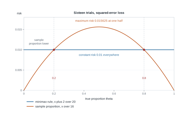
Step 5: compare, and refuse to declare a winner. The maximum risk of \(X/n\) is \(0.015625\) against \(0.01\), an improvement in the worst case of more than a third. But \(\theta(1 - \theta)/16 = 0.01\) exactly when \(\theta(1 - \theta) = 0.16\), that is at \(\theta = 0.2\) and \(\theta = 0.8\), so the sample proportion has lower risk whenever \(\theta\) is below \(0.2\) or above \(0.8\), and near the endpoints it wins by an enormous factor. Neither rule dominates; the sample proportion is itself admissible under this loss, a classical result proved by a limiting-Bayes argument this page does not develop.
Step 6: read the least favourable prior. \(\mathrm{Beta}(2, 2)\) is not vague; it is a mild hump centred at \(1/2\), where estimation is hardest, which is what “least favourable” means. On observing \(x = 3\) successes, \(X/n\) reports \(0.1875\) and \(\delta^{*}\) reports \(5/20 = 0.25\) — the price of the worst-case guarantee at a \(\theta\) that is probably small.
n     <- 16
theta <- seq(0, 1, length.out = 401)
risk_sample  <- theta * (1 - theta) / n
risk_minimax <- 1 / (4 * (sqrt(n) + 1)^2)

max(risk_sample)             # 0.015625, attained at theta = 1/2
risk_minimax                 # 0.01, whatever theta is
polyroot(c(0.16, -1, 1))     # 0.2 and 0.8, where the two risks agree

set.seed(2027)
one_run <- function(th) {
  x <- rbinom(20000, size = n, prob = th)
  c(sample = mean((x / n - th)^2), minimax = mean(((x + 2) / 20 - th)^2))
}
sapply(c(0.1, 0.2, 0.5, 0.8), one_run)
The misreading to avoid
The sentence to dismantle follows every conjugate calculation: “the Bayes estimator minimizes the risk, so it is better than the sample mean.” What a Bayes rule minimizes is the Bayes risk, one number obtained by averaging the risk curve against one prior; it does not minimize \(R(\theta, \cdot)\) at any fixed \(\theta\). In the first worked example it is worse than the sample mean at every \(\theta\) more than \(1.5\) units from the prior mean — most of the parameter space. Restore the quantifier — “the smallest prior-averaged risk among all rules, for this prior” — and the claim becomes true and much less impressive.
A second misreading attaches to Stein: “shrinkage improves the estimate of each coordinate, so shrink everything.” The theorem is about \(E_\theta \lVert \delta(X) - \theta \rVert^2\), a sum over coordinates, and an individual coordinate can be estimated worse: if nine offsets sit near zero and the tenth is far away, the common factor drags the tenth toward the centre and inflates its own squared error while the total still falls. If your loss is the error in one named coordinate the theorem says nothing in your favour, and at \(p = 1\) or \(p = 2\) the sample vector is admissible.
A third confuses the guarantees. A \(95\) per cent posterior interval describes the posterior given the data you have, under a prior you chose; a \(95\) per cent confidence interval describes a procedure’s long-run behaviour across repetitions. They can coincide numerically — let the prior variance grow in Step 2 above and the posterior interval converges to the frequentist one — but a posterior probability is neither a p-value nor a long-run error rate. If you want coverage, check coverage. And minimaxity is neither safety nor unimprovability: the binomial rule above is beaten across both tails, and the sample vector in \(p \ge 3\) dimensions is minimax and inadmissible at once.
When you read any claim of optimality, name the criterion, the loss, and the set the optimization ran over. “Best” with none of those three attached is not a statement about statistics.
Practice on your own
- Verify the crossing condition \((\theta - \mu)^2 < (1 + w)(\tau^2 + \sigma^2/n)\) algebraically, then track the width of the winning region as \(n\) grows with \(\tau\) fixed. Does the Bayes rule become safer or riskier relative to \(\bar{X}\), and does the risk difference behave the same way?
- Take a posterior that is Gamma with shape \(2\) and rate \(1\). Compute the Bayes action under squared error and under absolute error, and say what feature of the posterior opens the gap that the normal case closes.
- Repeat the constant-risk construction at \(n = 4\), \(n = 25\), and \(n = 100\), comparing the minimax risk \(1/\big(4(\sqrt{n} + 1)^2\big)\) with \(1/(4n)\). What happens to the minimax rule’s advantage in large samples, and why is that expected?
- Consider the weighted loss \(L(\theta, a) = (\theta - a)^2 / \big[\theta(1 - \theta)\big]\) for the same binomial model. Show that \(X/n\) has risk \(1/n\) at every \(\theta\) strictly inside \((0, 1)\), and explain why changing the loss changes which rule has constant risk without changing the model.
- Simulate the shrinkage claim below, checking the first two rows against \(10\) and the Poisson-mixture formula, and report a Monte Carlo standard error with each estimate.
set.seed(2027)
p <- 10
js      <- function(x, p) (1 - (p - 2) / sum(x^2)) * x
js_plus <- function(x, p) max(0, 1 - (p - 2) / sum(x^2)) * x

study <- function(len2, reps = 10000) {
  mu <- c(sqrt(len2), rep(0, p - 1))
  loss <- replicate(reps, {
    x <- rnorm(p, mean = mu, sd = 1)
    c(raw = sum((x - mu)^2), stein = sum((js(x, p) - mu)^2),
      positive = sum((js_plus(x, p) - mu)^2))
  })
  rbind(risk = rowMeans(loss), mcse = apply(loss, 1, sd) / sqrt(reps))
}
sapply(c(0, 4, 16, 64), function(v) study(v)["risk", ])
Where to read more
- Bayes rules, admissibility, complete classes, and the minimax argument used above are developed at graduate level in MIT OpenCourseWare 18.655 Mathematical Statistics, the place to see the measure-theoretic conditions in full.
- For the conjugate calculations under the worked examples, see Penn State STAT 415.
- The optional Hogg, McKean, and Craig alignment for this week is Chapter 8.5 together with Chapter 11. The book is optional and never required for this course; availability and licence terms for every source listed here remain unconfirmed.
- Both code blocks run in base R and
stats, with nothing installed beyond The R Project for Statistical Computing and Quarto. - Course pages: the notes overview, the syllabus, the schedule, and the resources page.
Where this goes next
This week closes the loop Week 1 opened. You now have three ways to compare procedures whose risk curves cross — average against a prior, examine the worst case, or check whether one sits entirely below another — and they disagree in a principled way.
Week 15 spends it: one inferential target carried through an exact procedure, a large-sample likelihood procedure, a resampling procedure, a rank-based procedure, and a Bayesian decision, with the five conclusions set side by side. The Bayesian route there is the one built here, so bring the habit with you — never report a posterior summary without saying what loss made it the right summary, and never accept a claim of optimality without asking which of this week’s three criteria it refers to. Use the notes overview to see where this unit sits in the arc from Week 13 onward.