Week 12 — Distribution-free inference and rank procedures
Where this week starts
Week 11 attacked an unknown sampling distribution by resampling: replace \(F\) by the empirical distribution \(F_n\) and trust the analogy. That trust is asymptotic, and you watched it fail outright for the sample maximum. This week takes the opposite route. Rather than estimate the unknown distribution, it builds statistics whose null distribution does not involve \(F\) at all — not approximately, not for large \(n\), but exactly, at every sample size, for every continuous \(F\) at once.
The device is deliberately crude: throw away the numerical values and keep only their ordering. If \(X_1, \dots, X_n\) are independent draws from a continuous \(F\), the vector of ranks is uniform over the \(n!\) orderings whatever \(F\) is, because the ordering survives any strictly increasing transformation and \(F\) itself is one. A statistic built from ranks alone therefore has a null distribution you compute by counting — literally: in this page’s examples it has 64 or 20 configurations, and you will list them.
Hold this week’s exactness beside Week 10’s. A randomization test is exact because the experimenter actually randomized, so an observational data set analysed with the same arithmetic inherits nothing. A rank test is exact because of an invariance in the model, and its validity is bought instead by assumptions — independence, continuity, and whichever symmetry the statistic needs. Neither is exact for free.
Three things should feel different by the end. “Distribution-free” should mean, precisely and only, that the null distribution of the statistic does not depend on \(F\); power does, and so does what a rejection means. The rank-sum test should have stopped being “the nonparametric \(t\) test” and become a test about the exceedance probability \(P(X > Y)\). And the price of ranks should be a number you can quote: against the \(t\) test at the normal model, an asymptotic relative efficiency of \(3/\pi\).
Why this matters beyond the theorem
Here is the claim this week has to stop. Two production lines are compared on a durability measure, a rank-sum test returns a p-value just under \(0.05\), and the report reads “the test shows line B is larger on average”. Now suppose the lines have exactly the same mean — one output roughly uniform, the other right-skewed with a long tail — and the exceedance probability is \(0.568\) rather than one half. The test is behaving correctly, the p-value is honest, and the report is false.
That is not carelessness about wording; it is not knowing what the procedure estimates. The rank-sum procedure’s functional is the exceedance probability, which equals one half neither exactly when the means agree nor exactly when the medians agree. Only an assumed shift model turns it into a location difference.
What you will be able to do
- Prove that the rank vector of an independent continuous sample is uniform over all orderings, and use that proof to say what “distribution-free” does and does not assert.
- Derive the exact null distributions of the sign and signed-rank statistics, naming the condition each derivation uses, and compute an exact p-value by enumeration.
- Derive the null moments of the rank-sum statistic from sampling ranks without replacement, and convert between the rank-sum and Mann-Whitney forms.
- Identify the exceedance probability as what a rank-sum procedure estimates, and state the extra assumption under which it becomes a difference in location.
- Compute asymptotic relative efficiencies against the \(t\) test at a stated density, and say what the bound \(108/125\) does and does not guarantee.
- Diagnose the failure of a rank procedure under asymmetry, unequal spread, or ties, and say what a reported level then means.
Terms and notation worth fixing
One convention holds throughout. In one-sample and paired problems \(n\) is the number of observations or pairs; in two-sample problems \(m\) and \(n\) are the two group sizes and \(N = m + n\).
| Symbol or term | Meaning as used in this course |
|---|---|
| \(F\), \(G\) | the continuous distributions generating the first and second samples; continuity is exactly what makes ties impossible with probability one |
| \(R_i\) | a rank within whichever set the surrounding text names — the pooled sample for the rank-sum statistic, the absolute differences for the signed-rank statistic |
| \(W^{+}\) | the signed-rank statistic: the sum of the ranks of those absolute differences whose sign is positive |
| \(W\) | the rank-sum statistic: the sum of the pooled ranks held by the first sample |
| \(U\) | the Mann-Whitney count of pairs with \(X_i > Y_j\), equal to \(W - m(m+1)/2\) |
| \(p\) | the exceedance probability \(P(X > Y)\), this week’s estimand — never a p-value, which is always written out in words |
| \(\Delta\) | the location shift in the model \(G(y) = F(y - \Delta)\), a quantity that exists only when that model is assumed |
| ARE | asymptotic relative efficiency: the limiting ratio of the sample sizes two tests need for the same power against the same local alternatives |
Ranks, exchangeability, and distribution-free null distributions
Everything this week rests on one proposition, so it is proved rather than quoted.
Proposition. Let \(X_1, \dots, X_n\) be independent with a common continuous distribution \(F\), and let \(R_i\) be the rank of \(X_i\) among the \(n\) values. Then with probability one the values are distinct, and the random permutation \((R_1, \dots, R_n)\) is uniform over the \(n!\) orderings, whatever \(F\) is.
Working. Continuity gives \(P(X_i = X_j) = 0\) for each of the finitely many pairs \(i \ne j\), so the ranks are almost surely a genuine permutation of \(1, \dots, n\). For uniformity, use exchangeability: because the \(X_i\) are independent and identically distributed, \((X_{\pi(1)}, \dots, X_{\pi(n)})\) has the same joint law as \((X_1, \dots, X_n)\) for every permutation \(\pi\). Every ordering is therefore as probable as every other, and since almost surely exactly one of the \(n!\) orderings occurs, each carries probability \(1/n!\). Independence and identical distribution gave exchangeability, continuity removed ties, and the shape of \(F\) never appeared.
A second route makes the invariance visible. Applying the nondecreasing \(F\) cannot change the ordering, and for continuous \(F\) the values \(F(X_i)\) are independent uniform variables on \((0, 1)\), so the sample’s rank vector is that of a uniform sample: every continuous \(F\) is carried to the same place. In the language of Week 6, the rank vector is a maximal invariant under strictly increasing transformations.
Why a rank vector forgets the shape
See the invariance on numbers before using it. Take five readings from group A, namely \(2.1, 3.4, 4.0, 5.2, 6.8\), and five from group B, namely \(3.9, 5.5, 7.1, 8.3, 9.0\). Pooling and ranking gives group A the ranks \(1, 2, 4, 5, 7\), so its rank sum is \(W = 19\). Now corrupt the largest group B reading from \(9.0\) to \(41.0\) — a transposed digit, a units error, a genuinely long tail. It is still the largest value, so it keeps rank \(10\), every other rank is untouched, the rank sum is \(19\) again, and the exact two-sided rank-sum p-value is \(24/252 = 0.095\) either way. Welch’s \(t\) statistic, which uses the spacings, moves from \(-2.01\) to \(-1.26\) and its p-value from \(0.081\) to \(0.275\).
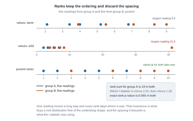
The moral runs both ways. Ranks buy a null distribution immune to the shape of \(F\) and to any one observation’s magnitude; ranks cost the spacing, which carries real information when the model is nearly right.
The sign test and its binomial null
The coarsest rank procedure keeps only whether each observation lies above or below a hypothesized value. Let \(X_1, \dots, X_n\) be independent from a continuous \(F\) with median \(\theta\), so \(F(\theta) = 1/2\). To test \(H_0: \theta = \theta_0\), count
\[B = \sum_{i=1}^{n} \mathbf{1}\{X_i > \theta_0\} .\]
Under \(H_0\) the indicators are independent and each is Bernoulli with success probability \(P(X_i > \theta_0) = 1 - F(\theta_0) = 1/2\), so \(B\) is binomial with \(n\) trials and probability one half — free of \(F\). The argument used only independence and the fact that \(\theta_0\) is a median of the continuous \(F\); it did not use symmetry, finite variance, or a shift model. This is the most assumption-light procedure in the course, with a correspondingly narrow null: a statement about one quantile and nothing else.
Discreteness returns exactly as in Week 4. At \(n = 6\) the attainable one-sided tail probabilities are \(1/64\), \(7/64\), \(22/64\) and upward, so an exact test of size \(0.05\) does not exist and the largest attainable level at or below \(0.05\) is \(1/64 \approx 0.0156\). Either accept the conservatism or restore exact size by randomizing on the boundary as in Week 2 — but do not call the conservative test a test of size \(0.05\).
The signed-rank statistic and the symmetry it needs
The sign test throws away too much: it cannot tell small positive differences from large ones. The Wilcoxon signed-rank statistic keeps the ordering of the magnitudes as well. Let \(D_1, \dots, D_n\) be independent paired differences from a continuous distribution, let \(R_i\) be the rank of \(\lvert D_i \rvert\) among the absolute differences, and set
\[W^{+} = \sum_{i=1}^{n} R_i \, \mathbf{1}\{D_i > 0\} .\]
The hypothesis this statistic is distribution-free under is not “the median of \(D\) is zero”; it is the stronger statement that \(D\) is symmetric about zero, and that extra strength is what the derivation consumes. Under symmetry and continuity, \(\lvert D_i \rvert\) and \(\operatorname{sign}(D_i)\) are independent and the sign is equally likely either way. Now write \(Z_r\) for the sign indicator of the difference whose absolute value has rank \(r\). Every rank is a function of the absolute differences alone, so the \(Z_r\) inherit that independence, and
\[W^{+} = \sum_{r=1}^{n} r \, Z_r , \qquad Z_1, \dots, Z_n \text{ independent Bernoulli with probability } 1/2 ,\]
an identity in which no unknown distribution appears. All \(2^n\) sign patterns are equally likely, so the null distribution comes from listing the subsets of \(\{1, \dots, n\}\) and recording their sums. The moments follow, using \(\sum r = n(n+1)/2\), \(\sum r^2 = n(n+1)(2n+1)/6\), and independence of the \(Z_r\) for the variance:
\[E_0 W^{+} = \sum_{r=1}^{n} \frac{r}{2} = \frac{n(n+1)}{4}, \qquad \operatorname{Var}_0 W^{+} = \sum_{r=1}^{n} \frac{r^2}{4} = \frac{n(n+1)(2n+1)}{24} .\]
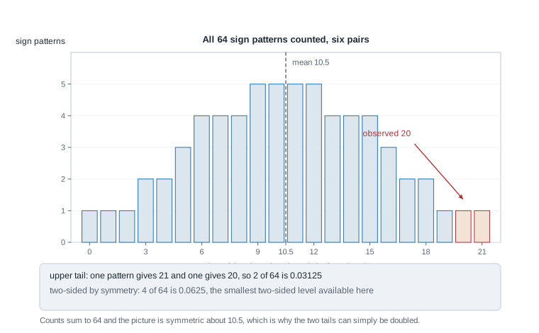
At \(n = 6\) these give a mean of \(10.5\) and a variance of \(546/24 = 22.75\).
Say what breaks if symmetry is dropped. If the differences are skewed with median zero, the signs are no longer independent of the magnitudes — large absolute differences tend to carry the sign of the long tail — so the representation fails, the enumerated distribution is not the null distribution, and the actual size can sit well away from the nominal level. The sign test survives that case and the signed-rank test does not: each step up in efficiency is bought with a step up in what the null hypothesis asserts.
What the rank-sum test actually estimates
Let \(X_1, \dots, X_m\) come from a continuous \(F\) and \(Y_1, \dots, Y_n\) from a continuous \(G\), all independent, and take \(H_0: F = G\). Under that null the \(N = m + n\) pooled observations are exchangeable, so each of the \(\binom{N}{m}\) rank assignments to the first sample is equally likely.
From pooled ranks to the Mann-Whitney count
Let \(W\) be the sum of the pooled ranks held by the \(X\) sample. Under \(H_0\) those ranks are a simple random sample of size \(m\) drawn without replacement from \(\{1, \dots, N\}\), which is all the moment calculation needs. That population has mean \((N+1)/2\) and variance \((N^2 - 1)/12\), and such a sample sum has variance \(m \cdot \frac{N - m}{N - 1} \cdot \frac{N^2 - 1}{12}\); put \(N - m = n\) and cancel \(N - 1\):
\[E_0 W = \frac{m(N+1)}{2}, \qquad \operatorname{Var}_0 W = \frac{mn(N+1)}{12} .\]
The Mann-Whitney form is the same statistic recentred. Counting pairs in which an \(X\) exceeds a \(Y\) gives \(U = \#\{(i, j) : X_i > Y_j\}\), and because the \(X\) ranked \(k\)-th within its own sample exceeds exactly its pooled rank minus \(k\) of the \(Y\) values, summing over \(k\) yields \(U = W - m(m+1)/2\).
That identity turns a rank sum into an estimand. Since \(E[\mathbf{1}\{X_i > Y_j\}] = P(X > Y)\) for every pair and there are \(mn\) pairs, \(E[U] = mn \, p\) with \(p = P(X > Y)\) — under the alternative as much as under the null, with no shift model and no equal-shape assumption. So \(\hat{p} = U/(mn)\) estimates the exceedance probability without bias, and the rank-sum test is the test of \(p = 1/2\) that comes with it. Under \(H_0: F = G\) we do get \(p = 1/2\); the converse fails, since many pairs of distinct distributions have exceedance probability exactly one half — and, in the other direction, a pair can agree exactly on the mean while \(p\) sits well away from one half, as below.
Only under a shift model \(G(y) = F(y - \Delta)\) does \(p\) become a monotone function of a location difference, with \(p = 1/2\) exactly when \(\Delta = 0\). Under that assumption the test inverts, by the duality of Week 4, into the Hodges-Lehmann interval for \(\Delta\), whose point estimate is the median of the \(mn\) pairwise differences \(Y_j - X_i\). Say plainly which world you are in: without the shift model, an honest estimate of an exceedance probability; with it, a location statement resting on an assumption nobody checked.
Efficiency: what ranks cost and what they buy
Comparing a rank test with the \(t\) test needs the local alternatives of Week 6, because at any fixed alternative both powers tend to one and the comparison is empty. Fix \(\theta_n = \theta_0 + h/\sqrt{n}\), which holds the problem at constant difficulty as \(n\) grows, and define the asymptotic relative efficiency as the limiting ratio of sample sizes needed for equal power against it. For a location problem with density \(f\), median \(\theta\), and finite variance \(\sigma^2\),
\[\mathrm{ARE}(\text{Wilcoxon}, t) = 12 \sigma^2 \left( \int f^2(x) \, dx \right)^{2}, \qquad \mathrm{ARE}(\text{sign}, t) = 4 \sigma^2 f(\theta)^{2} .\]
Both require \(\sigma^2 < \infty\), since the \(t\) test’s own limit does. Against a Cauchy model there is no ratio to report — the comparison degenerates rather than the rank test becoming infinitely good.
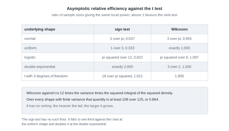
Read the table as a price list. At the normal model the Wilcoxon procedures return \(3/\pi = 0.955\), so they need about five per cent more observations than the \(t\) test for the same local power: a small premium. At the double exponential they need only two-thirds as many, and at a \(t\) model with three degrees of freedom the ratio is \(75/(4\pi^2) \approx 1.900\). The floor is the striking part: over every shape with finite variance the Wilcoxon efficiency is at least \(108/125 = 0.864\), attained at one particular parabolic density, and there is no matching ceiling. The sign test has no such floor — a third as efficient at the uniform shape — because it discards magnitudes entirely.
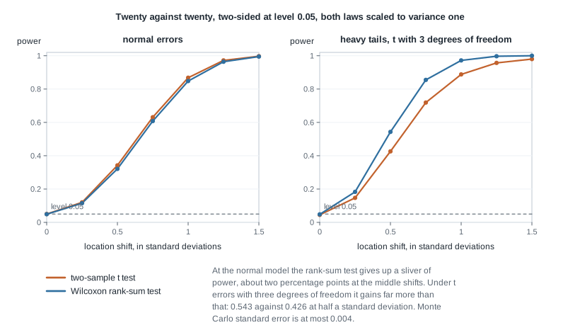
Confirm the asymptotics at a sample size someone might actually have. The design behind the figure: twenty per group, two-sided tests at level \(0.05\), both error laws scaled to variance one, and twenty thousand replicates.
set.seed(2027)
power_at <- function(shift, n = 20, reps = 20000, heavy = FALSE) {
  draw <- function(k) if (heavy) rt(k, df = 3) / sqrt(3) else rnorm(k)
  hits <- replicate(reps, {
    x <- draw(n); y <- draw(n) + shift
    c(t.test(x, y)$p.value, wilcox.test(x, y)$p.value) < 0.05
  })
  rowMeans(hits)
}
At a shift of half a standard deviation the normal panel reads \(0.342\) for the \(t\) test against \(0.321\) for the rank-sum; the heavy-tailed panel reverses it decisively, \(0.426\) against \(0.543\). The Monte Carlo standard error is at most \(0.0036\), so a fresh run moves each entry by a few thousandths and by nothing that changes either comparison. Both tests also hold their level at zero shift — the finite-sample check to make before reading any power claim.
Worked example — the signed-rank test on six paired readings
Six specimens are measured before and after a treatment on a clinical laboratory instrument, in coded units. The differences are modelled as independent draws from a continuous distribution symmetric about \(\theta\), and the question is whether \(\theta = 0\).
Step 1. The differences. After minus before gives \(0.7,\; 2.4,\; -0.3,\; 1.9,\; 3.1,\; 1.2\). Their absolute values are all distinct, so there are no ties and the enumeration below is the exact null distribution, not an approximation to it.
Step 2. Rank the magnitudes.
| Difference \(D_i\) | \(0.7\) | \(2.4\) | \(-0.3\) | \(1.9\) | \(3.1\) | \(1.2\) |
|---|---|---|---|---|---|---|
| \(\lvert D_i \rvert\) | \(0.7\) | \(2.4\) | \(0.3\) | \(1.9\) | \(3.1\) | \(1.2\) |
| Rank \(R_i\) | \(2\) | \(5\) | \(1\) | \(4\) | \(6\) | \(3\) |
| Sign | \(+\) | \(+\) | \(-\) | \(+\) | \(+\) | \(+\) |
Step 3. The statistic. Adding the ranks carrying a positive sign, \(W^{+} = 2 + 5 + 4 + 6 + 3 = 20\), and the negative side is \(W^{-} = 1\). As a check the two must sum to \(6 \cdot 7/2 = 21\), and they do.
Step 4. The exact one-sided p-value, by counting. All \(2^6 = 64\) sign patterns are equally likely under the null, so the one-sided p-value is the fraction of subsets of \(\{1, \dots, 6\}\) summing to at least \(20\). Exactly two do: the whole set, summing to \(21\), and \(\{2, 3, 4, 5, 6\}\), summing to \(20\). Any other subset omits some element other than the smallest and so falls to \(19\) or below. The p-value is \(2/64 = 0.03125\).
Step 5. Two-sided. The null distribution is symmetric about \(n(n+1)/4 = 10.5\), so the lower tail at or below \(W^{-} = 1\) holds the same two configurations and doubling gives \(4/64 = 0.0625\). At the conventional level the one-sided test rejects and the two-sided test does not. That is discreteness, not paradox, and not a licence to switch tests after the fact: the attainable two-sided p-values here are \(2/64\), \(4/64\), \(6/64\) and upward, so the smallest available is \(0.03125\).
d <- c(0.7, 2.4, -0.3, 1.9, 3.1, 1.2)
r <- rank(abs(d))
w_plus <- sum(r[d > 0])                          # 20
patterns <- as.matrix(expand.grid(rep(list(c(0, 1)), 6)))
null_w <- patterns %*% seq_len(6)                # all 64 equally likely values
mean(null_w >= w_plus)                           # 0.03125
Step 6. The neighbours on the same data. The sign test sees only that five of six differences are positive, so its two-sided p-value is \(2 \times 7/64 = 0.21875\) — nowhere near rejection, having discarded that the one negative difference is also the smallest in magnitude. The paired \(t\) test uses the spacings: the mean difference is \(1.5\) with sample standard deviation \(1.2247\), so the standard error is \(1.2247/\sqrt{6} = 0.5\) exactly, \(t = 3.00\) on five degrees of freedom, and the two-sided p-value is \(0.0301\).
The signed-rank result licenses a one-sided statement at level \(0.03125\) that the difference distribution is not symmetric about zero, given that it is symmetric about something. It licenses no claim about the size of the effect; for that, invert the test to the Hodges-Lehmann estimate, the median of the \(21\) Walsh averages \((D_i + D_j)/2\) with \(i \le j\), which here equals \(1.55\). Nor does it support the reading that the \(t\) test found an effect the rank test missed: with six pairs the exact test has only 64 atoms, and no evidence whatever pushes its two-sided p-value below \(0.03125\).
The same reasoning, transferred
Move the counting argument to two independent samples of three, three plants of each of two varieties in a field trial, so \(m = n = 3\) and \(N = 6\). Under \(H_0: F = G\) the ranks \(1, \dots, 6\) split between the groups in \(\binom{6}{3} = 20\) equally likely ways, and \(W\), the rank sum of the first group, runs from \(1 + 2 + 3 = 6\) to \(4 + 5 + 6 = 15\). Listing the twenty triples gives counts \(1, 1, 2, 3, 3, 3, 3, 2, 1, 1\) at the values \(6\) through \(15\): symmetric about \(E_0 W = m(N+1)/2 = 10.5\), with variance \(mn(N+1)/12 = 5.25\).
What stayed the same is the whole logic — an exchangeability argument makes a finite set of configurations equally likely, and the p-value is a count over the size of that set. What changed is the set: sign patterns of a paired design become group assignments of a two-sample design, and \(64\) becomes \(20\). The consequence is sharper here. The most extreme outcome, one group holding the three smallest ranks, has one-sided p-value \(1/20 = 0.05\) and two-sided \(0.10\), so no three-against-three data set can reach a two-sided exact p-value below \(0.10\). The shortage is of configurations, and no choice of statistic repairs it.
Second worked example — a rank-sum comparison with equal means
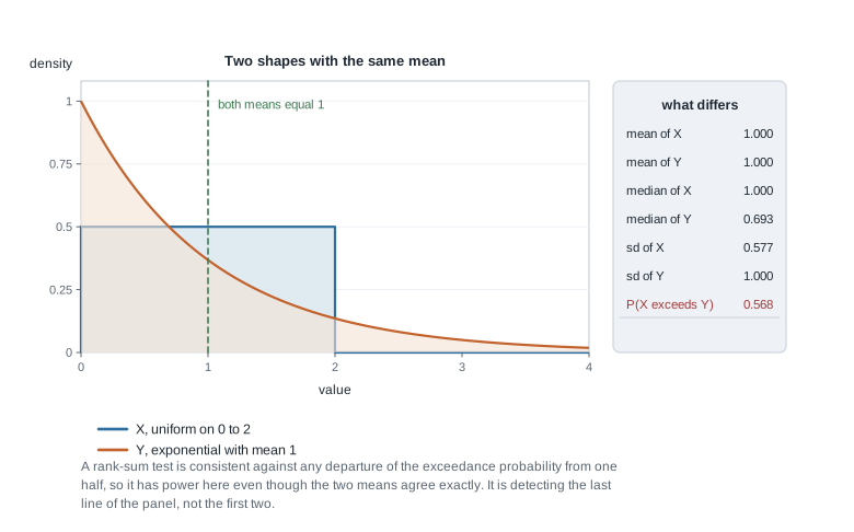
This example exercises calibration rather than derivation: what does a rank-sum rejection mean when the distributions differ in shape but not in mean? Take \(X\) uniform on \((0, 2)\), a supplier whose coded lifetimes are tightly bounded, and \(Y\) exponential with mean one, a supplier with a long tail. Both means equal \(1\), and no \(\Delta\) makes \(G(y) = F(y - \Delta)\), so the shift model is false here.
The estimand, exactly. Condition on \(X\) and integrate:
\[p = P(X > Y) = E_X\big[ P(Y < X \mid X) \big] = E_X\big[ 1 - e^{-X} \big] = 1 - \frac{1}{2}\int_0^2 e^{-x} \, dx = 1 - \frac{1 - e^{-2}}{2} = \frac{1 + e^{-2}}{2} .\]
Since \(e^{-2} = 0.13534\), this is \(p = 0.56767\). The medians differ, \(1\) against \(\ln 2 = 0.693\), and so do the standard deviations, \(2/\sqrt{12} = 0.577\) against \(1\). The mean is the one summary that agrees, and the mean is the one summary the rank-sum test is not about.
A stated data set. A reliability test runs forty units from each supplier and yields \(U = \#\{X_i > Y_j\} = 1006\) of the \(mn = 1600\) pairs, so \(\hat{p} = 1006/1600 = 0.629\), above the true \(0.568\) but well within sampling variability. Under \(H_0: F = G\),
\[E_0 U = \frac{mn}{2} = 800, \qquad \operatorname{Var}_0 U = \frac{mn(N+1)}{12} = \frac{1600 \cdot 81}{12} = 10800 ,\]
so the null standard deviation is \(\sqrt{10800} = 103.92\) and the standardized statistic is \((1006 - 800)/103.92 = 1.98\). The two-sided normal-approximation p-value is \(0.047\), or \(0.048\) with a continuity correction of one half; either way the test rejects at the conventional level. In rank-sum form this is \(W = U + m(m+1)/2 = 1826\) against a null mean of \(1620\), the same \(206\) units.
What the \(t\) test says. The sample means are \(1.02\) and \(0.99\) with sample standard deviations \(0.57\) and \(0.95\), so Welch’s standard error is \(\sqrt{0.57^2/40 + 0.95^2/40} = \sqrt{1.2274/40} = 0.175\), giving \(t = 0.03/0.175 = 0.17\) and a two-sided p-value near \(0.86\). The two procedures disagree completely and neither is wrong.
What has been detected. The test has rejected \(p = 1/2\), and \(p\) really is \(0.568\); the rank-sum test is consistent against any fixed departure from one half, so at forty per group it has genuine power. It has not detected a difference in means, because there is none. The defensible sentence is this: a component drawn at random from supplier A outlasts one drawn at random from supplier B with estimated probability \(0.63\), while the two average lifetimes are indistinguishable. That is what a customer comparing two units cares about, and it is not about location.
One caution belongs here. The exact level is guaranteed under \(H_0: F = G\), not under equality of means or medians. If equality of medians is your hypothesis and the shapes or spreads differ, this test does not have level \(\alpha\) for it — the distribution-free analogue of the Behrens-Fisher problem, showing up as a rejection like this one.
The misreading to avoid
The sentence to dismantle, in the form graduate students actually write it: “the Wilcoxon rank-sum test is the nonparametric version of the \(t\) test, so it compares the medians of the two groups without making any assumptions.” Three claims, and all three fail.
“Without any assumptions.” The test assumes independence within and between samples, and continuity — without which ties occur with positive probability, the enumerated distribution is not the null distribution, and the usual correction changes the variance. Its exact level is a guarantee about the single hypothesis \(F = G\). Distribution-free is a statement about the null distribution of the statistic and nothing more; power depends on \(F\) heavily.
“Compares the medians.” It does not, and no assumption-free procedure could. Let \(X\) be uniform on \((-1, 1)\), and let \(Y\) be the mixture that is uniform on \((-4, 0)\) with probability one half and uniform on \((0, 1/2)\) with probability one half. Both medians are exactly \(0\). On the first branch \(Y \le -1\) with probability \(3/4\) and then \(X > Y\) certainly, while for \(Y\) uniform on \((-1, 0)\), \(P(X > Y \mid Y = y) = (1 - y)/2\) averages to \(3/4\); that branch contributes \(3/4 + (1/4)(3/4) = 15/16\). On the second branch \((1 - y)/2\) averages to \(3/8\). Hence
\[p = \tfrac{1}{2} \cdot \tfrac{15}{16} + \tfrac{1}{2} \cdot \tfrac{3}{8} = \tfrac{15}{32} + \tfrac{6}{32} = \tfrac{21}{32} = 0.65625 .\]
Equal medians, and an exceedance probability of nearly two-thirds. A rank-sum test on large samples from this pair rejects with probability approaching one, and it is right to.
“The nonparametric version of the \(t\) test.” The two procedures target different functionals, so they are not two routes to one conclusion. They agree only inside the shift model, and that model is a real assumption — arguably stronger than normality, since it constrains the entire shape of both distributions to match. If you want to compare means, test means: a \(t\) procedure, a permutation test on the difference in means from Week 10, or a bootstrap interval from Week 11. If the exceedance probability is your question, say so in those words.
One quieter misreading is worth naming. Because rank tests are unaffected by outliers they get called robust in next week’s sense. They are resistant, which is not the same: a rank procedure bounds the influence of a wild value by discarding the information in every value, and changes the estimand to do it.
Practice on your own
- Derive \(\operatorname{Var}_0 W^{+} = n(n+1)(2n+1)/24\) from \(W^{+} = \sum_r r Z_r\), saying where independence of the \(Z_r\) enters, then enumerate at \(n = 6\) and confirm the variance is \(22.75\).
- Enumerate the signed-rank null distribution at \(n = 5\), where there are \(32\) sign patterns, and find the smallest attainable two-sided p-value. How many pairs are needed before an exact two-sided level of at most \(0.01\) becomes attainable?
- Construct a pair of continuous distributions with the same mean, the same median, and exceedance probability different from one half — or prove no such pair exists — then simulate to check.
- Simulate the size of the rank-sum test when \(F\) and \(G\) are normal with a common mean but standard deviations \(1\) and \(3\), at \(m = n = 15\), over twenty thousand replicates. Is the rejection rate near \(0.05\), and what does that imply for testing equality of medians?
- Verify by integration that \(\mathrm{ARE}(\text{sign}, t)\) equals \(2/\pi\) at the standard normal and \(2\) at the double exponential density \(\tfrac{1}{2} e^{-\lvert x \rvert}\), and state which feature of the double exponential makes the sign test win.
Where to read more
Start with the course material and go outward only as far as you need.
- The optional Hogg, McKean, and Craig alignment for this week is Chapter 10.1 through 10.5, covering the sign, signed-rank, and rank-sum procedures with their efficiency comparisons. The text is optional throughout this course and is never required to be purchased.
- MIT OpenCourseWare 18.655 Mathematical Statistics treats testing and asymptotic efficiency at this level; its material on local alternatives is the right companion to the efficiency section above.
- Penn State STAT 415 gives a slower first pass at the sign and rank tests with more small-sample examples to work.
- The R Project for Statistical Computing documents the base functions used above, and Quarto is the authoring system this draft site is built in. Availability and licence terms are stated by those sources rather than here.
- The course pages: the notes overview, the syllabus, the schedule, and the resources overview.
- This unit leans directly on Week 10, for exact tests built by enumeration, and Week 11, for the resampling alternative.
Where this goes next
Rank procedures answer “what if I do not know the shape” by discarding the values and keeping the ordering, which buys an exact null distribution and moves the estimand. Week 13 asks something narrower: keep the target roughly where it was, and make the procedure’s behaviour continuous in the underlying distribution, so a small contamination of \(F\) moves the estimate and its standard error only a little. Its instruments are the influence function, the breakdown point, and M-estimation, and this page’s efficiency arithmetic reappears there as the price of bounded influence. Continue to Week 13, or return to the notes overview.