Week 10 — Randomization, permutation, and exact conditional inference
Where this week starts
Every test you have built so far borrowed its null distribution from a model. In Week 2 the null distribution of \(\bar{X}\) came from the normal family you assumed; in Week 5 the chi-square reference came from regularity conditions on a likelihood. Each time, “under the null, the statistic has this distribution” followed from assumptions about how the numbers were generated, and when those assumptions failed the calibration failed with them.
This week the null distribution comes from somewhere else entirely: the randomizer the experimenter actually used. If you assigned three of six coupons to a coating by drawing labels out of a hat, you know — not assume, know — that each of the twenty possible splits had probability one in twenty. That knowledge is enough to build an exact reference distribution for any statistic you like, with no claim about the shape of the response distribution. The price is a null hypothesis stronger than the one you may have had in mind, and a reference set whose size is fixed by the design and therefore limits how small a p-value can ever be.
Three ideas carry the week and they are not the same idea. The first is the randomization distribution: the statistic recomputed over every assignment the design could have produced, with the observed responses held fixed. The second is the permutation test as used outside designed experiments, where the same arithmetic is justified instead by exchangeability — a real assumption, in the same sense that normality is one. The third is exact conditional inference, where a nuisance parameter is eliminated by conditioning on a sufficient statistic, which is how Fisher’s exact test acquires a hypergeometric null with no unknown parameter in it. All three lead to counting rather than to a limit theorem, and by the end the word “exact” should read as a statement about the level of a procedure — not a promise that the size equals \(\alpha\), that the p-value is precise, or that the test has any power at all.
Why this matters beyond the theorem
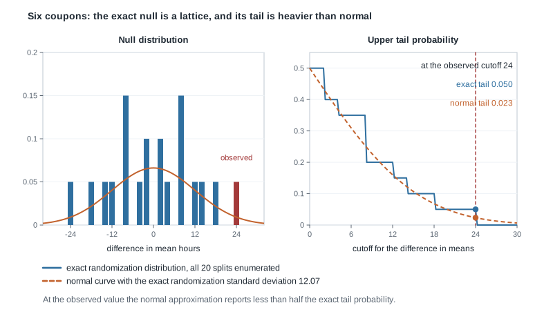
Here is the stake. A laboratory runs a small trial on six specimens, three per group, and reports a significant result at level 0.05 from a normal-theory two-sample test. Redo the arithmetic the way the design licenses, by enumerating all twenty ways the coating could have been assigned, and the two-sided p-value is 0.10 — the smallest value a three-against-three design can produce. The approximation made no arithmetic error; it answered a question about a normal population nobody had sampled, and at the observed value its tail was less than half the exact one.
The reverse error is quieter and more common. Someone takes two groups that were never assigned to anything — patients who happened to receive one drug or another — shuffles the labels ten thousand times, and reports the result as “distribution-free, so assumption-free”. The shuffling asserts that under the null every relabelling was equally likely. That is an assumption about the world, and when treatment was chosen rather than assigned it is usually false. The arithmetic is identical; the warrant is gone.
What you will be able to do
Work through this page and the week’s problem workshop and you should be able to do the following.
- Derive the randomization distribution of a stated statistic from a stated assignment mechanism, by enumeration when the reference set is small enough to list.
- State the sharp null of no effect for any unit, distinguish it from the null of no average effect, and say which one a randomization test tests.
- Prove that the randomization p-value satisfies \(P(p \le \alpha) \le \alpha\), and identify the step of that proof that fails when the assignment distribution is not the one the reference set was built from.
- Compute an exact conditional p-value for a two-by-two table by hypergeometric counting, and give the two arguments — design randomization and conditioning on a sufficient statistic — that lead to the same law.
- Diagnose the discreteness of a small reference set: list the attainable levels and give the actual size of a test at nominal level 0.05.
- Distinguish Monte Carlo error, which more sampled permutations remove, from statistical uncertainty, which they do not.
Terms and notation worth fixing
Every symbol below carries the meaning fixed here for the rest of the page.
| Symbol | What it means on this page |
|---|---|
| \(Y_i(1)\), \(Y_i(0)\) | The two potential responses of unit \(i\), under treatment and under control: fixed numbers attached to the unit, not random variables |
| \(W\) | The assignment vector, with \(W_i = 1\) when unit \(i\) is treated; the only random object in sight |
| \(\mathcal{W}\), \(M\) | The reference set of assignments the design can produce, and how many there are. For three of six units, \(M = 20\) |
| Sharp null | The hypothesis \(Y_i(1) = Y_i(0)\) for every unit \(i\): no effect on anyone, not merely none on average |
| \(T(w, y)\) | The statistic recomputed at assignment \(w\) with the observed response vector \(y\) held fixed |
| \(\alpha\) | Level, as in Week 2: an upper bound on the probability of rejecting a true null |
| \(A\) | Successes among the treated units of a two-by-two table, with both margins fixed |
| \(\psi\) | The odds ratio of that table; both nulls considered here set \(\psi = 1\) |
The randomization distribution as the reference
Fix a finite set of units \(i = 1, \dots, N\). Attach to each unit two fixed numbers, \(Y_i(1)\) and \(Y_i(0)\), the response it would show under treatment and under control. Nothing about them is random: they are properties of the unit and the two conditions, fixed before any coin is flipped. The experiment produces an assignment vector \(W\), and the response you observe for unit \(i\) is \(Y_i = W_i Y_i(1) + (1 - W_i) Y_i(0)\) — the one potential outcome the assignment revealed.
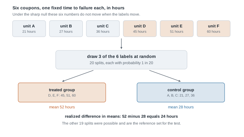
Read the figure before the algebra. The six numbers at the top belong to the units; the box in the middle is the design, a device with a known distribution over splits; the two groups at the bottom are what one turn of that device produced. Everything this week does follows from taking that middle box seriously as the source of randomness.
Potential outcomes and the sharp null
The sharp null is \(H_0 : Y_i(1) = Y_i(0)\) for every unit \(i\). If treatment changes nothing for anybody, unit \(i\) shows the same number whichever group it lands in, so the observed response vector \(y\) is a fixed list attached to the units and you can compute what the statistic would have been under any other assignment \(w\). Write that quantity \(T(w, y)\). Without the sharp null it does not exist: under a null that only fixes the average effect, moving unit \(i\) from control to treatment changes its response by an unknown amount, and there is nothing to recompute.
That is why the sharp null is not a technicality. It is stronger than the null of no average effect, \(\frac{1}{N}\sum_i \{Y_i(1) - Y_i(0)\} = 0\), which is satisfied by a treatment that helps half the units and harms the other half equally. A randomization test can reject the sharp null in that situation while the average effect is exactly zero, and it would be right to: the sharp null is false. The honest report says the test found evidence of some effect on some unit, not evidence of a positive mean effect. There is a known repair when the mean is the target — permute a studentized statistic rather than the raw difference in means — which keeps exactness under the sharp null and adds asymptotic validity under the weaker one; this page states that repair without developing it.
Why the test is exact, and what exact means
Let \(W\) be drawn uniformly from \(\mathcal{W}\), the set of \(M\) assignments the design admits, and let \(t_{\text{obs}} = T(W, y)\) be the realized statistic. The randomization p-value is the share of the reference set at least as extreme:
\[ p = \frac{1}{M} \, \# \{ w \in \mathcal{W} : T(w, y) \ge t_{\text{obs}} \}. \]
Proposition. Under the sharp null, with \(W\) uniform on \(\mathcal{W}\) and \(y\) therefore fixed, \(P(p \le \alpha) \le \alpha\) for every \(\alpha \in (0, 1)\).
Working. Write \(G(w) = \#\{w' \in \mathcal{W} : T(w', y) \ge T(w, y)\}\), so that \(p = G(W)/M\). Fix \(\alpha\), put \(k = \lfloor \alpha M \rfloor\), and let \(\mathcal{A} = \{w : G(w) \le k\}\) be the assignments that would produce a p-value at or below \(\alpha\). The claim is that \(\mathcal{A}\) has at most \(k\) elements. Suppose it had \(k + 1\), and among those take the one with the smallest statistic value, \(w^{*}\). All \(k + 1\) have values at least \(T(w^{*}, y)\), so \(G(w^{*}) \ge k + 1 > k\), contradicting \(w^{*} \in \mathcal{A}\). Hence \(P(p \le \alpha) = \#\mathcal{A} / M \le k/M \le \alpha\). The argument used no distributional assumption whatever, only that \(W\) is uniform on the set the reference distribution was built over.
Three consequences deserve to be stated separately. First, exactness is a statement about level: the test that rejects when \(p \le \alpha\) has size at most \(\alpha\), and the size is the largest attainable p-value not exceeding \(\alpha\). Second, the attainable p-values are multiples of \(1/M\), so a small design has a coarse grid; that is a fact about the experiment, not the analysis, and no software choice repairs it. Third, the proof breaks at its first line if \(W\) was not drawn from the distribution used to build \(\mathcal{W}\) — if the technician quietly gave the coating to the specimens that looked sturdier, the reference set is a fiction and the guarantee goes with it.
The variance of the difference in means over the reference set can also be written down exactly, a useful check on any enumeration. For a completely randomized design with \(n_1\) treated and \(n_2\) control units, \(N = n_1 + n_2\), and \(D(w)\) the difference in group means, the sharp null gives \(E\{D(W)\} = 0\) and
\[ \operatorname{Var}\{D(W)\} = S^2 \left( \frac{1}{n_1} + \frac{1}{n_2} \right), \qquad S^2 = \frac{1}{N-1}\sum_{i=1}^{N} (y_i - \bar{y})^2 . \]
The derivation is finite-population sampling, not distribution theory: \(D\) is an affine function of the total of a simple random sample of size \(n_1\) drawn without replacement from the \(N\) fixed numbers, and that total has variance \(n_1 (1 - n_1/N) S^2\). Note what is absent: no normality, no independence across units, no model for the responses.
Conditioning to remove a nuisance parameter
The second route to an exact test starts from a model rather than a design, and removes what it does not want to estimate. Suppose \(X_1 \sim \text{Binomial}(n_1, \theta_1)\) and \(X_2 \sim \text{Binomial}(n_2, \theta_2)\) independently, and the null of interest is homogeneity, \(H_0 : \theta_1 = \theta_2 = \theta\) with the common value unknown. Week 6 gave the general lesson: a composite null carrying an unknown nuisance parameter rarely admits an exact test unless the nuisance can be eliminated. Here it can, because under \(H_0\) the total \(S = X_1 + X_2\) is sufficient for \(\theta\).
From the design to the hypergeometric law
Condition on \(S = s\) and compute. Under the null,
\[ \begin{aligned} P(X_1 = a, S = s) &= \binom{n_1}{a} \theta^{a}(1-\theta)^{n_1 - a} \binom{n_2}{s-a}\theta^{s-a}(1-\theta)^{n_2-s+a} \\ &= \binom{n_1}{a}\binom{n_2}{s-a} \, \theta^{s} (1-\theta)^{N-s}, \end{aligned} \]
and summing over \(a\) with Vandermonde’s identity gives \(P(S = s) = \binom{N}{s}\theta^{s}(1-\theta)^{N-s}\). Dividing,
\[ P(X_1 = a \mid S = s) = \frac{\binom{n_1}{a}\binom{n_2}{s-a}}{\binom{N}{s}}, \qquad \max(0, s - n_2) \le a \le \min(n_1, s), \]
which is the hypergeometric law and carries no unknown parameter. The conditioning did exactly one job: it removed \(\theta\). If the null is instead a fixed odds ratio \(\psi\), the same calculation returns the noncentral hypergeometric law with weights \(\binom{n_1}{a}\binom{n_2}{s-a}\psi^{a}\), so the conditional test is a test about \(\psi\) and nothing else.
A completely randomized experiment with a binary response reaches the same distribution without any sampling model. Under the sharp null each unit’s success or failure is fixed in advance, so the total number of successes is a constant of the data, the number of treated units is a constant of the design, and the treated group is a simple random sample of size \(n_1\) from \(N\) units of which \(s\) are successes: the count of treated successes is hypergeometric by construction. Both margins are fixed for you rather than by you, and the much-argued question of whether it is legitimate to condition on them does not arise in the randomized case at all.
What sampled permutations cost
When \(M\) is too large to enumerate — a two-group comparison with twelve units per group already has \(\binom{24}{12} = 2{,}704{,}156\) assignments — draw \(B\) of them at random, independently and uniformly, and estimate. The estimator to use is
\[ \hat{p}_B = \frac{1 + \#\{b \le B : T(W_b, y) \ge t_{\text{obs}}\}}{B + 1}, \]
with the observed value counted in both the numerator and the denominator. The plus-one is not a fudge. Under the sharp null the observed assignment and the \(B\) draws are exchangeable, so \(t_{\text{obs}}\) is no more likely to lead the list of \(B + 1\) values than any other member of it, and rejecting when \(\hat{p}_B \le \alpha\) has size at most \(\alpha\) for every finite \(B\). The naive proportion, which divides by \(B\) and can equal zero, has no such guarantee.
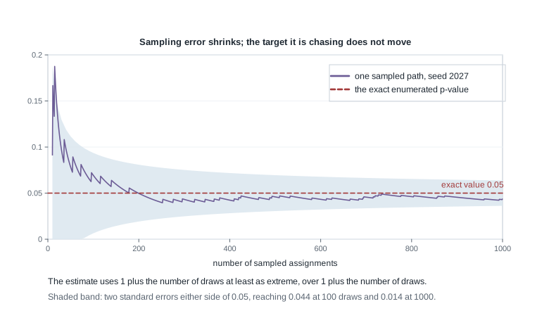
The figure runs this estimator on the six-coupon example, where the exact value 0.05 is known by enumeration, so the sampling error is visible rather than hypothetical. The band has half-width \(2\sqrt{p(1-p)/B}\), which is 0.044 at \(B = 100\) and 0.014 at \(B = 1000\). Sampling more assignments narrows that band and nothing else; it never narrows the uncertainty that comes from having six units, which the coarseness of the reference set already told you about. Report the number of draws beside any sampled p-value near a decision boundary.
Worked example — six coupons, every split enumerated
A bench trial exposes six metal coupons to a corrosive bath and records the hours until a fixed level of pitting appears. Three of the six were assigned the experimental coating by drawing labels, so all \(\binom{6}{3} = 20\) splits had probability one in twenty. The realized data, in hours, are: coated 45, 51, 60 and uncoated 21, 27, 36. All data on this page are illustrative.
Step 1. State the null and check that it makes the arithmetic possible. The sharp null says every coupon would have failed at exactly its observed hour under either condition, so the six numbers 21, 27, 36, 45, 51, 60 are fixed and any split can be scored.
Step 2. Score the observed split. Take \(T\) to be the difference in group means. Coated: \((45 + 51 + 60)/3 = 52\). Uncoated: \((21 + 27 + 36)/3 = 28\). So \(t_{\text{obs}} = 52 - 28 = 24\) hours.
Step 3. Enumerate. Score all twenty splits. Because the two groups are the same size, swapping a split’s labels negates its statistic, so the values come in ten opposite pairs and the reference set is exactly symmetric about zero. The distinct values, with how many splits give each, are \(\pm 24\), \(\pm 18\), \(\pm 14\), \(\pm 12\) and \(\pm 4\) once each, \(\pm 2\) twice each, and \(\pm 8\) three times each — ten positive and ten negative, twenty in all.
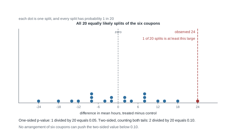
Step 4. Count. Exactly one split — the realized one — gives a difference of at least 24, so the one-sided p-value is \(1/20 = 0.05\). Counting both tails, two splits have \(|T| \ge 24\), so the two-sided p-value is \(2/20 = 0.10\).
y <- c(21, 27, 36, 45, 51, 60)      # the six fixed responses, in hours
treated <- c(4, 5, 6)               # the split that actually happened
diff_in_means <- function(idx) mean(y[idx]) - mean(y[-idx])
reference <- apply(combn(6, 3), 2, diff_in_means)
observed <- diff_in_means(treated)
mean(reference >= observed)              # 0.05, which is 1/20 exactly
mean(abs(reference) >= abs(observed))    # 0.10
What this licenses. At level 0.05 the one-sided test rejects the sharp null, and the guarantee behind that is the design, not a normal approximation. What it does not license. Nothing at all at level 0.05 two-sided: the reference set is symmetric, so two-sided p-values are even multiples of \(1/20\), the smallest attainable is 0.10, and a two-sided test at that level rejects for no data set whatever. The rejection also says nothing about the size of the effect; turning the test into an interval means inverting it over a family of sharp nulls with a stated constant effect, which is Week 4’s duality argument applied here.
The variance formula gives \(S^2 = 1092/5 = 218.4\) and \(\sqrt{218.4 \times (1/3 + 1/3)} = \sqrt{145.6} = 12.07\) hours, matching the enumerated values. Feeding 24 into a normal reference with that standard deviation gives an upper tail of 0.023, less than half the exact 0.05.
The same reasoning, transferred
Change the design and the logic does not change. Suppose the same laboratory works with five matched pairs of panels, coating one member of each pair by a fair coin toss made independently within each pair. The within-pair differences, coated minus uncoated in hours, come out as \(+31\), \(+14\), \(+26\), \(-8\), \(+20\).
Under the sharp null the five absolute differences \(31, 14, 26, 8, 20\) are fixed and only their signs were random, so the reference set is the \(2^5 = 32\) equally likely sign vectors. The observed sum is \(31 + 14 + 26 - 8 + 20 = 83\) and the absolute differences total 99. Flipping a subset of signs to negative reduces the sum by twice that subset’s total, so \(T \ge 83\) requires the flipped subset to total at most \((99 - 83)/2 = 8\). Only the empty subset and the single value 8 qualify, so two of the thirty-two sign vectors are at least as extreme and the one-sided p-value is \(2/32 = 0.0625\); the two-sided count is four, giving 0.125.
d <- c(31, 14, 26, -8, 20)
flips <- as.matrix(expand.grid(rep(list(c(1, -1)), 5)))
reference_pairs <- as.vector(flips %*% abs(d))
mean(reference_pairs >= sum(d))     # 2/32 = 0.0625
What stayed the same: the sharp null, the fixing of the responses it delivers, the statistic, the counting rule, and the exactness proposition, which never mentioned what \(\mathcal{W}\) was. What changed is \(\mathcal{W}\) itself, and with it the grid of attainable levels — multiples of \(1/32\) rather than \(1/20\). Worth noticing: a completely randomized design on these same ten panels would have had \(\binom{10}{5} = 252\) assignments, a much finer grid. Pairing gave that up for a statistic whose reference distribution is far more tightly concentrated, and the trade pays only when the members of a pair resemble each other.
Second worked example — a two-by-two table by exact conditional counting
Twelve seedlings are randomized six to a treated tray and six to a control tray, and each is scored after four weeks as vigorous or not. The counts came out like this.
| Group | Vigorous | Not vigorous | Total |
|---|---|---|---|
| Treated | 5 | 1 | 6 |
| Control | 1 | 5 | 6 |
| Total | 6 | 6 | 12 |
The observed odds ratio is \((5 \times 5)/(1 \times 1) = 25\), and the expected counts under homogeneity are 3 in every cell, small enough that the chi-square approximation of Week 5 has no business being used here.
Step 1. Fix the margins and identify the reference set. Six treated units is the design; six vigorous seedlings in total is a consequence of the sharp null, which fixes each seedling’s score. The table is therefore determined by \(A\), the number of vigorous seedlings among the treated, and \(A\) can be \(0, 1, \dots, 6\): seven tables in all.
Step 2. Get the null distribution by counting. Under the sharp null the treated group is a simple random sample of six from twelve units, six of which are vigorous, so \(P(A = a) = \binom{6}{a}\binom{6}{6-a} / \binom{12}{6}\) with \(\binom{12}{6} = 924\). The seven numerators are \(1, 36, 225, 400, 225, 36, 1\), which sum to 924 as Vandermonde’s identity promises.
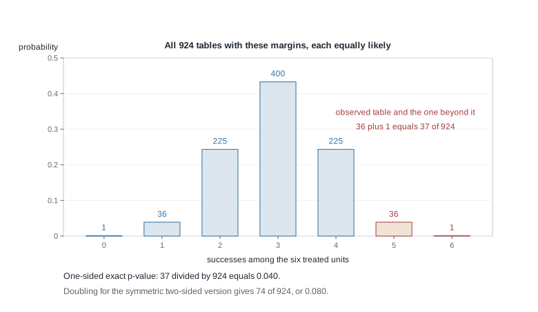
Step 3. Count the tail. Tables at least as extreme in the direction of the alternative are \(a = 5\) and \(a = 6\), with \(36 + 1 = 37\) of the 924, so the one-sided exact p-value is \(37/924 = 0.040\). The distribution is symmetric here because the two group sizes and the two response totals are equal, so the two-sided value by either doubling or by summing the tables no more probable than the observed one is \(74/924 = 0.080\).
sum(dhyper(5:6, m = 6, n = 6, k = 6))   # 0.04004329, which is 37/924
fisher.test(matrix(c(5, 1, 1, 5), 2, 2), alternative = "greater")$p.value
Step 4. Read the calibration honestly. The attainable upper-tail p-values with these margins are \(1/924 = 0.0011\), then \(37/924 = 0.040\), then \(262/924 = 0.284\). The test that rejects when \(p \le 0.05\) therefore has size 0.040, not 0.05: it is conservative, and the shortfall of one percentage point is the price of discreteness, exactly as the Clopper-Pearson interval of Week 4 paid it. Notice also that the conclusion concerns \(\psi\) and the sharp null; it is not a statement about a risk difference, and with six units per arm it is not a precise statement about anything.
The misreading to avoid
Here is the sentence to dismantle, said out loud every semester: “A permutation test makes no assumptions, so it is the safe choice whenever I am unsure about normality — and since it only shuffles labels, I can run it on any two groups I have.”
Three things are wrong with it. First, the shuffling is a claim, not a neutral operation. In the coupon trial the reference set and its probabilities are those of the randomizer that was actually used. For two groups that arrived already formed, permuting labels asserts that under the null every relabelling was equally likely, which is exchangeability of the pooled sample — an assumption about the world of exactly the same logical type as normality, merely a different one. Where treatment was chosen rather than assigned, sicker patients getting the aggressive drug, it is false, and the permutation p-value inherits the same confounding a normal-theory test would.
Second, the null being tested moves when the justification moves. Under exchangeability, the hypothesis that makes the reference set correct is equality of the two whole distributions, not of two means, so a rejection can be produced by a difference in spread with the means identical; Week 12 will show a rank procedure doing precisely that. Under randomization the null is sharper still: no effect on any single unit. Neither null is “the means are equal”, so no report should claim a mean difference without the extra argument.
Third, “exact” is not “powerful” and not “precise”. Exactness says the size does not exceed the nominal level. It says nothing about how often the test rejects when it should, and in a small design it is compatible with never rejecting at all: the three-against-three design had a smallest attainable two-sided p-value of 0.10. Nor is the number precise — sampled permutations add Monte Carlo error, and a coarse reference set allows few values. State the size of the reference set beside every exact p-value.
Practice on your own
These are for your own checking; the calibration lab goes further.
- Rerun the six-coupon enumeration with the uncoated readings unchanged and the coated readings 39, 44, 52. Score all twenty splits, count the tail, and report both p-values. Then check the variance formula against the variance of your twenty enumerated values.
- Show that for a completely randomized design with \(n_1 = n_2\) the reference set of the difference in means is symmetric about zero, and deduce that the attainable two-sided p-values are even multiples of \(1/M\). Then find the smallest equal-group design, in total units, for which a two-sided randomization test can reject at level 0.05.
- Construct potential outcomes for four units under which the average treatment effect is exactly zero but the sharp null is false. Say what a randomization test that rejects has discovered, and write the sentence you would put in a report.
- Take the two-by-two table with six treated, six control, and five vigorous seedlings in total. List the admissible tables, compute the hypergeometric probabilities, and give the exact size of the one-sided test at nominal level 0.05. Compare it with the size found above.
- Simulate the sampled-permutation estimator on the coupon data with \(B = 50\), repeated a thousand times, and plot the spread of \(\hat{p}_B\) around the exact 0.05. Then explain why the naive proportion can return zero and why that is not a valid p-value.
Where to read more
Read the open references for a second account of these arguments; the textbook alignment is in words below.
- MIT OpenCourseWare 18.655 Mathematical Statistics — a more measure-theoretic account of exact tests and of conditioning on a sufficient statistic.
- Penn State STAT 415 Introduction to Mathematical Statistics — a gentler treatment of the hypergeometric distribution and small-sample exact procedures, useful if the counting arguments here went quickly.
- The R Project for Statistical Computing and Quarto — everything shown here runs in base R with
stats, and the calibration lab is a Quarto document. - The optional Hogg, McKean, and Craig alignment for this week is Chapter 4.8, with Chapter 10 read as a preview of the distribution-free procedures Week 12 develops. The book is optional and these notes stand on their own; availability and licence terms for every source remain unconfirmed.
- Course pages: the notes overview, the syllabus, the schedule, and the resources page.
Where this goes next
Week 9 asked what many tests do to error control; this week asked where a single test’s null distribution comes from when no model supplies one. Week 11 keeps the resampling machinery and changes its target: the bootstrap resamples the data to approximate the sampling distribution of an estimator, a different object from the randomization distribution of a statistic under a null. Watch that distinction: a permutation test is exact under a stated mechanism, while a bootstrap interval is an approximation whose coverage must be checked.
The thread also runs to Week 12, where rank procedures turn out to be permutation tests whose statistic was chosen so the enumeration could be done once and tabulated for everyone. To revisit where this week’s exactness came from, reread Week 4 on inverting exact tests, and return to the notes overview for how the second half fits together.