Week 4 — Confidence-test duality, pivots, and exact procedures
Where this week starts
Weeks 2 and 3 built tests and asked how well they perform. A test settles one question at a time: is this value of \(\theta\) consistent with the data at level \(\alpha\)? What a reader of a scientific report wants instead is the whole collection of values that survive, and whether it reaches past whatever value the argument turns on. You already own the machinery for that. A confidence set is not a second theory bolted on beside testing; it is one family of tests, run at every candidate value at once and reported by listing which candidates survived.
Week 3 left something this reframing settles. Karlin-Rubin gave a uniformly most powerful one-sided test under monotone likelihood ratio, and the two-sided normal-mean problem had no such test at all. Both facts transfer intact, because an interval inherits the optimality of the tests you invert: the one-sided case yields a best interval and the two-sided case does not, for the same reason it failed there.
The week’s second job is to take the word exact seriously. In the normal model with unknown variance you can build an interval whose coverage is \(0.95\) for every mean and variance at every sample size. In a binomial model you cannot, because a non-randomized test’s size moves in jumps, and the best guarantee available is that coverage is at least nominal. What should feel different by the end is your reading of “a 95 percent confidence interval”: you should hear a claim about a procedure over repetitions, name the family of tests it inverts, and be able to compute its actual coverage.
Why this matters beyond the theorem
Here is the stake, in the smallest honest example available. Ten units go on a reliability test and three fail. The reflex procedure reports \(0.3\) plus or minus \(1.96\) estimated standard errors, the interval from \(0.016\) to \(0.584\). Run that procedure across all values of the true failure probability at twenty units and its actual coverage averages \(0.898\), sinking to \(0.639\) where the failure probability is small — precisely where a reliability study lives. Had zero units failed, the same recipe would return the interval from \(0\) to \(0\): certainty that the failure probability is exactly zero, from ten observations.
The opposite failure is quieter. The exact binomial interval never undercovers, but at ten trials its coverage averages \(0.984\), so it is wider than the advertised level requires and the test it inverts has less power than level \(0.05\) entitles it to. Both failures share one missing habit: quoting a nominal level without asking what the procedure actually does.
What you will be able to do
- State and prove the duality between a family of level-\(\alpha\) acceptance regions and a \(1 - \alpha\) confidence set, and name every condition the proof uses.
- Construct a confidence set by inverting a stated test family, showing the algebra that turns the acceptance inequality into endpoints, and say what makes the set an interval.
- Verify that a proposed quantity is pivotal, and explain why a pivot permits exact inversion while an approximate pivot does not.
- Derive the exact interval for a binomial proportion by inverting exact tests, and compute its actual coverage by enumeration rather than simulation.
- Diagnose whether a procedure is conservative, anti-conservative, or calibrated, and say what each behaviour costs.
- Distinguish coverage as a repeated-sampling property from the decision a single realized interval supports.
Terms and notation worth fixing
| Symbol or term | What it means on this page |
|---|---|
| \(A(\theta_0)\) | Acceptance region: the data values for which the test of \(H_0 : \theta = \theta_0\) does not reject |
| \(C(x)\) | Confidence set, a subset of \(\Theta\) determined by the data value \(x\) and random only through \(x\) |
| Coverage at \(\theta\) | \(P_\theta\{\theta \in C(X)\}\), the chance under \(\theta\) that the random set contains that same \(\theta\) |
| Nominal, actual | Nominal is the coverage requested; actual is what the procedure delivers |
| Conservative | Actual coverage at least nominal everywhere; anti-conservative means below nominal somewhere |
| \(Q(X, \theta)\) | A pivotal quantity: a function of data and parameter whose law is the same for every \(\theta\) |
| \(\beta_{\theta'}(\theta)\) | Power at \(\theta\) of the test whose null value is \(\theta'\); the family is indexed by its null value |
From acceptance regions to confidence sets
Fix a model \(\{P_\theta : \theta \in \Theta\}\) and let \(X\) be the data, in a sample space \(\mathcal{X}\). A map \(C\) from \(\mathcal{X}\) to subsets of \(\Theta\) is a \(1 - \alpha\) confidence set when \(P_\theta\{\theta \in C(X)\} \ge 1 - \alpha\) for every \(\theta \in \Theta\). Read that slowly: \(\theta\) appears three times and is a fixed constant in all three, the only random object is \(C(X)\), and the requirement is imposed at each \(\theta\) separately, so it is a family of statements.
The correspondence, stated and proved
Theorem (duality). Suppose for every \(\theta_0 \in \Theta\) a set \(A(\theta_0) \subseteq \mathcal{X}\) satisfies \(P_{\theta_0}\{X \in A(\theta_0)\} \ge 1 - \alpha\), so the non-randomized test rejecting \(H_0 : \theta = \theta_0\) when \(X \notin A(\theta_0)\) has level \(\alpha\). Define \[ C(x) = \{\theta \in \Theta : x \in A(\theta)\} . \] Then \(C\) is a \(1 - \alpha\) confidence set. Conversely, if \(C\) has coverage at least \(1 - \alpha\) and \(A(\theta_0) = \{x : \theta_0 \in C(x)\}\), then rejecting when \(X \notin A(\theta_0)\) is a level-\(\alpha\) test of \(H_0 : \theta = \theta_0\).
Working. Fix any \(\theta\) and compare two subsets of \(\mathcal{X}\): \[ \{x : \theta \in C(x)\} = \{x : x \in A(\theta)\} = A(\theta) . \] The first equality is the definition of \(C\) read backwards: membership of \(\theta\) in \(C(x)\) was defined to mean membership of \(x\) in \(A(\theta)\). Identical events have identical probabilities, so \(P_\theta\{\theta \in C(X)\} = P_\theta\{X \in A(\theta)\} \ge 1 - \alpha\), and \(\theta\) was arbitrary. The converse reverses the same two lines.
The proof is bookkeeping about one subset of \(\mathcal{X} \times \Theta\), namely \(S = \{(x, \theta) : x \in A(\theta)\}\): slice \(S\) at fixed \(\theta\) for an acceptance region, at fixed \(x\) for a confidence set.
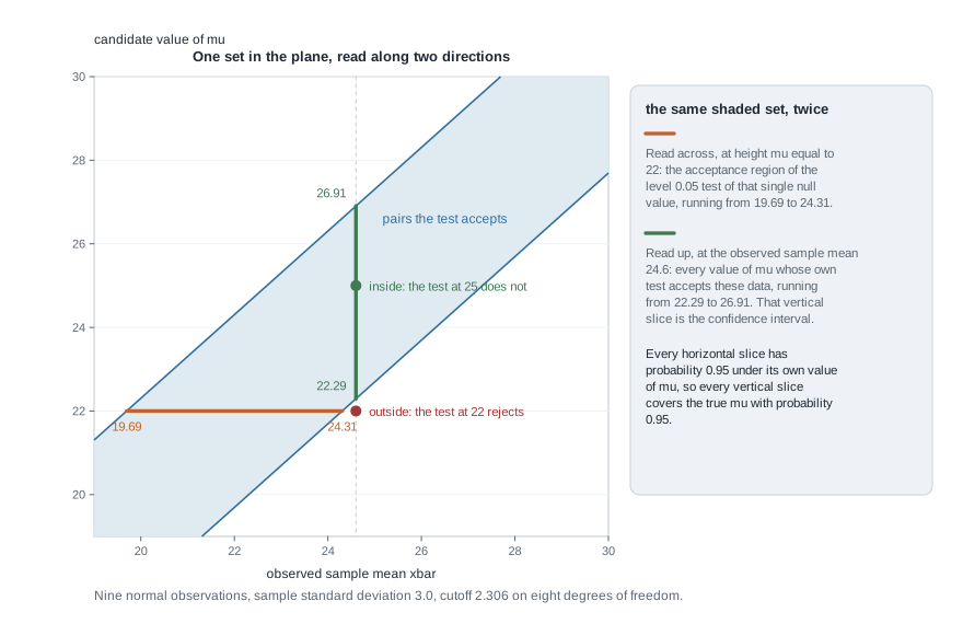
A short proof hides its conditions, so list them. A test must be supplied for every \(\theta_0\); one test gives one point, not an interval. The level requirement is evaluated at the null value itself, which is what makes the slice at \(\theta\) carry probability \(1 - \alpha\) under \(P_\theta\) and not under some other measure. And the tests must be non-randomized, so \(A(\theta_0)\) is a genuine set. Nothing else enters, measurability aside: no independence, no identical distribution, no exponential family, no smoothness, no large sample size, no assumption about the shape of \(\Theta\).
The third condition repays attention, because Week 2 showed a discrete model often needs a randomized test to attain size \(\alpha\) exactly. Such a test has no acceptance region — it rejects with probability \(\varphi(x)\) strictly between zero and one at some \(x\) — so what inverts is a random set depending on an auxiliary uniform draw, whose coverage holds only averaged over that draw. Almost nobody reports endpoints that depend on a coin flip, and that refusal is what makes exact discrete intervals conservative below.
One consequence imports Week 3 wholesale. For \(\theta \ne \theta'\), \[ P_\theta\{\theta' \in C(X)\} = P_\theta\{X \in A(\theta')\} = 1 - \beta_{\theta'}(\theta) , \] so the probability of covering a false value is one minus the power of that value’s own test. Making a set rarely cover wrong values and making its tests powerful are one problem stated twice. Inverting uniformly most powerful tests therefore minimizes the probability of covering each false value, over the alternatives those tests are most powerful against — the uniformly most accurate set — and where Week 3 found no such test, there is no such set either, with unbiasedness the same repair.
Pivots, and why inversion is easy when you have one
Inversion is solvable in principle and unpleasant in practice: you must generally work out \(A(\theta)\) separately for every \(\theta\). A pivot collapses that to one calculation. A pivotal quantity is a function \(Q(X, \theta)\) of data and parameter whose distribution under \(P_\theta\) is the same for every \(\theta\), nuisance components included. It is not a statistic — you cannot compute it without knowing \(\theta\) — and that is the point: it carries \(\theta\) inside it, so a probability statement about \(Q\) rearranges into one about \(\theta\).
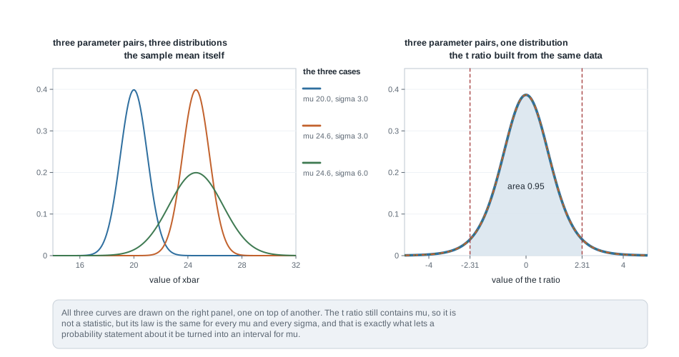
The left panel shows the sampling distribution of \(\bar{X}\) from nine normal observations under three parameter pairs: it moves and changes width, so no fixed cutoffs serve all of them. The right panel shows \(T = \sqrt{n}(\bar{X} - \mu)/S\) under those same three pairs. All three curves are drawn there; you see one, because they coincide. That is why a single number, \(2.306\), serves the whole family.
Such coincidences come from group structure. Write \(X_i = \mu + \sigma Z_i\) with \(Z_1, \dots, Z_n\) independent standard normal. Then \(\bar{X} - \mu = \sigma \bar{Z}\) and \(S = \sigma S_Z\), so \(T = \sqrt{n}\,\bar{Z}/S_Z\), in which no parameter appears. The argument needs the location-scale form and the normality of \(Z\), never the values of \(\mu\) and \(\sigma\).
Given a pivot, choose \(q_1 \le q_2\) with \(P\{q_1 \le Q \le q_2\} = 1 - \alpha\) under that common law. Then \(A(\theta) = \{x : q_1 \le Q(x, \theta) \le q_2\}\) has probability exactly \(1 - \alpha\) under every \(P_\theta\), and duality hands you \(C(x) = \{\theta : q_1 \le Q(x, \theta) \le q_2\}\). Two choices stay open. The pair \((q_1, q_2)\) is not determined: equal tails give the shortest interval when the pivot’s density is symmetric and unimodal, and generally not otherwise — the chi-square pivot below is a case in point. And whether \(C(x)\) is an interval depends on \(\theta \mapsto Q(x, \theta)\) being continuous and strictly monotone for each \(x\); when it is, the endpoints solve the two boundary equations, and when it is not, the set can be disconnected or unbounded. Fieller’s construction for a ratio of two normal means is the classical instance, where the set is sometimes the whole real line — an honest report that a small denominator leaves the ratio unconstrained.
What the correspondence does not promise
Duality is exact about level and silent about everything else. Four silences matter.
It does not promise that \(C(x)\) is an interval, is bounded, or is non-empty. An empty confidence set is not a contradiction: the requirement constrains how often the set misses the true \(\theta\), so a procedure may return nothing for some data provided that happens with probability at most \(\alpha\) under every \(\theta\). Nor does it say anything about width or power — the family that never rejects has level \(\alpha\) for any \(\alpha\) and inverts to \(C(x) = \Theta\), coverage one and no content.
It does not turn coverage into a statement about \(\theta\): the probability lives on the data at a fixed parameter value and does not become a distribution over parameter values. And it preserves what the tests actually have, not what they were asked for. If discreteness forces true size \(0.021\) when you asked for \(0.05\), the inverted set has coverage \(0.979\). Duality is faithful; it was the family that was approximate.
Exactness in a discrete model and the price of it
That last point deserves an identity rather than a sentence. Let \(\text{size}(\theta)\) be the actual rejection probability, under \(P_\theta\), of the family member whose null value is \(\theta\). Failing to cover \(\theta\) and rejecting that member are the same event, so \[ \text{coverage}(\theta) = 1 - \text{size}(\theta) \quad \text{for every } \theta \in \Theta . \] Everything Week 2 established about attainable sizes reappears here as coverage sitting above nominal.
Why a lattice-valued statistic cannot attain the level
Take \(X \sim \text{Binomial}(n, \theta_0)\) and a non-randomized test. Its rejection probability is a sum of finitely many binomial point masses, so as the critical count moves by one the size jumps by a whole mass rather than sliding. Hitting \(\alpha\) exactly would be a coincidence. Make that concrete with \(n = 10\), \(\theta_0 = 0.5\), tested two-sidedly with equal tails. Under the null \(X\) is symmetric about five and \(2^{10} = 1024\), so the attainable two-sided sizes are \[ 2P(X \le 0) = \frac{2}{1024} = 0.00195, \qquad 2P(X \le 1) = \frac{22}{1024} = 0.02148, \qquad 2P(X \le 2) = \frac{112}{1024} = 0.10938 , \] using \(\binom{10}{0} = 1\), \(\binom{10}{1} = 10\), \(\binom{10}{2} = 45\). The largest not exceeding \(0.05\) is \(0.02148\), so the level-\(0.05\) test of \(\theta = 0.5\) at ten trials really has size \(0.021\), and by the identity the inverted interval covers \(0.5\) with probability \(0.979\). A randomized test would close the gap exactly, rejecting at \(x = 2\) and \(x = 8\) with a probability chosen to reach \(0.05\), at the cost of endpoints depending on an auxiliary draw. Conservatism is what you pay for endpoints that are a function of the data alone.
What conservatism buys and what it costs
It buys a guarantee with no fine print: coverage at least \(1 - \alpha\) at every \(\theta\) and every \(n\), with no approximation and no sample size below which the claim quietly fails. It costs width, and with it power.
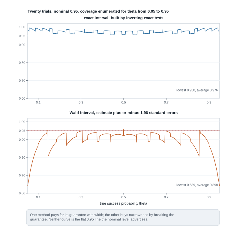
Both curves come from enumerating all twenty-one outcomes at each \(\theta\), so they carry no Monte Carlo error. Over true proportions from \(0.05\) to \(0.95\) the exact interval averages \(0.976\) coverage and never drops below \(0.958\), while the Wald interval averages \(0.898\) and reaches down to \(0.639\). Neither is the flat line at \(0.95\) that a nominal level suggests. A third construction sits between them: the score interval, obtained by inverting the score test, averages \(0.954\) over that range with a low of \(0.917\). It is far better calibrated than either and gives up the guarantee, dipping below \(0.95\) in places.
Two cautions before concluding that conservative means safe. At twenty trials and a true proportion of \(0.3\) the expected width is \(0.413\) for the exact interval against \(0.364\) for the score interval, so the guarantee costs about \(0.05\) of expected width and the dual test loses the matching power. And a procedure delivering \(0.98\) is not usable inside a calculation that assumes \(0.95\): wrong operating characteristics propagate whichever way they point.
Worked example — inverting the t test for a normal mean
The model and the question. A clinical laboratory measures a calibration standard nine times. Model the measurements as \(X_1, \dots, X_9\) independent \(N(\mu, \sigma^2)\) with both parameters unknown, and suppose the sample mean is \(\bar{x} = 24.6\) and the sample standard deviation is \(s = 3.0\); these numbers are illustrative. Which values of \(\mu\) are consistent with the data at level \(0.05\), reached by inversion rather than by quoting a formula?
Step 1, the family of tests. For each candidate \(\mu_0\) use \(T(\mu_0) = \sqrt{n}(\bar{X} - \mu_0)/S\) and reject \(H_0 : \mu = \mu_0\) when \(|T(\mu_0)| > t_{8, 0.975} = 2.306\). That test needs three facts: independence and normality give \(\bar{X} \sim N(\mu, \sigma^2/n)\) exactly, \((n-1)S^2/\sigma^2 \sim \chi^2_{n-1}\) exactly, and \(\bar{X}\) independent of \(S^2\). Together they make \(T(\mu_0)\) a \(t\) variable on \(n - 1 = 8\) degrees of freedom under the null, and all three need normality, not merely finite variance.
Step 2, the level is exact and uniform. Because \(T(\mu)\) is pivotal, \(P_{\mu, \sigma}\{|T(\mu)| \le 2.306\} = 0.95\) for every pair \((\mu, \sigma)\), so every member of the family has size exactly \(0.05\) and duality delivers coverage exactly \(0.95\), not merely at least.
Step 3, invert. The acceptance region for \(\mu_0\), and the set it inverts to, are \[ A(\mu_0) = \left\{ x : \left| \frac{\sqrt{n}(\bar{x} - \mu_0)}{s} \right| \le 2.306 \right\} , \qquad C(x) = \left\{ \mu : |\bar{x} - \mu| \le 2.306 \, \frac{s}{\sqrt{n}} \right\} . \] The set is an interval because \(\mu \mapsto T(x, \mu)\) is continuous and strictly decreasing, so \(|T| \le 2.306\) carves out one connected stretch whose endpoints are where \(T\) equals \(\pm 2.306\).
Step 4, the numbers. Here \(s/\sqrt{n} = 3.0/3 = 1.0\) exactly, so the half-width is \(2.306\) and \[ C(x) = (24.6 - 2.306,\; 24.6 + 2.306) = (22.294,\; 26.906) . \]
Step 5, interval and tests agree. They must, being one procedure, but look at how narrowly.
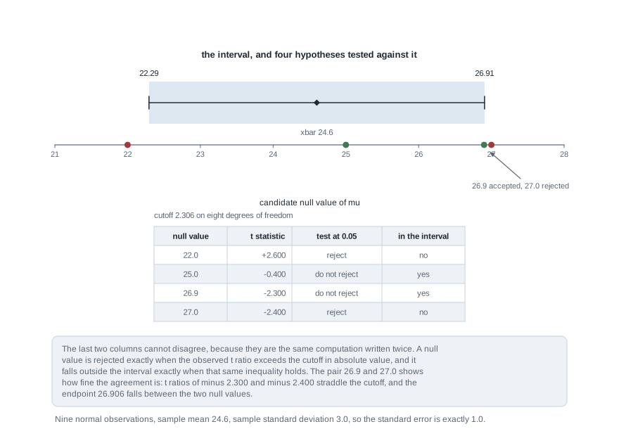
At \(\mu_0 = 22\) the ratio is \((24.6 - 22)/1.0 = 2.600\), exceeding \(2.306\), so the test rejects and \(22\) sits outside. At \(\mu_0 = 25\) the ratio is \(-0.400\) and \(25\) sits inside. The interesting pair is \(26.9\) and \(27.0\), with ratios \(-2.300\) and \(-2.400\): the first accepted, the second rejected, and the endpoint \(26.906\) falls between them, as it must.
xbar <- 24.6; s <- 3.0; n <- 9
tcrit <- qt(0.975, df = n - 1)                 # 2.306004
xbar + c(-1, 1) * tcrit * s / sqrt(n)          # 22.294  26.906
abs((xbar - c(22, 25, 26.9, 27)) / (s / sqrt(n))) > tcrit
What this licenses, and what it does not. You may say the procedure producing \((22.294, 26.906)\) covers the true mean in \(95\) percent of repetitions of this experiment, whatever \(\mu\) and \(\sigma\) are, and that every \(\mu_0\) outside those endpoints would have been rejected at level \(0.05\). You may not say the probability that \(\mu\) lies between \(22.294\) and \(26.906\) is \(0.95\): both endpoints and \(\mu\) are now numbers, and the statement is true or false. It does not hold \(95\) percent of measurements either; a prediction interval for one future measurement is far wider. And the coverage is exactly \(0.95\) only under normality; with heavy-tailed measurement error at nine observations it is something else, which is Week 13’s subject.
The same reasoning, transferred
Change the model, keep the structure. Ten units in a reliability test have independent exponential lifetimes with rate \(\lambda\), totalling \(\sum x_i = 15.0\) time units. The pivot is \(Q = 2\lambda\sum_i X_i\): each \(\lambda X_i\) is exponential with rate one, the sum has the gamma law with shape ten and rate one, and doubling a gamma variable with shape \(k\) and rate one gives a chi-square variable on \(2k\) degrees of freedom, so \(Q \sim \chi^2_{20}\) whatever \(\lambda\) is. With equal tails, \(\chi^2_{20, 0.025} = 9.591\) and \(\chi^2_{20, 0.975} = 34.170\), so \[ C(x) = \{\lambda : 9.591 \le 2\lambda(15.0) \le 34.170\} = \left( \frac{9.591}{30}, \; \frac{34.170}{30} \right) = (0.3197, \; 1.139) . \]
What stayed the same: a pivot, a probability statement free of the parameter, and an inversion that yields an interval because \(\lambda \mapsto 2\lambda \sum x_i\) is continuous and strictly increasing. What changed is instructive: the chi-square law is skewed, so the interval is not symmetric about \(\hat\lambda = 10/15 = 0.667\) — it reaches \(0.347\) below and \(0.472\) above — and equal tails no longer give the shortest interval. And because confidence sets are exactly equivariant under a monotone reparameterization, the interval for the mean lifetime \(\mu = 1/\lambda\) comes from transforming the endpoints and swapping them, \((1/1.139, 1/0.3197) = (0.878, 3.128)\), coverage still exactly \(0.95\). That equivariance is free here and is not free for the Wald intervals of Week 5.
Second worked example — the exact interval for a binomial proportion
The model and the question. Ten independent units go on test and three fail, so model the count as \(X \sim \text{Binomial}(10, \theta)\) with \(\theta\) the failure probability. There is no pivot: \(X\) is discrete and its law depends on \(\theta\) in a way no transformation removes. Inversion still works, value by value, but its coverage will be conservative rather than exact, and this example is about what that costs.
Step 1, the test family. For each candidate \(\theta_0\), reject \(H_0 : \theta = \theta_0\) when either tail probability at the observed count is small: \[ P_{\theta_0}(X \ge x) \le 0.025 \qquad \text{or} \qquad P_{\theta_0}(X \le x) \le 0.025 . \] The two conditions cannot both hold, since \(P_{\theta_0}(X \ge x) + P_{\theta_0}(X \le x) \ge 1\), so the size is a sum of two disjoint tail probabilities each at most \(0.025\) and the test has level \(0.05\) — with actual size usually strictly less, by the counting above.
Step 2, invert, and check the set is an interval. Duality gives \(C(x) = \{\theta : P_\theta(X \ge x) > 0.025 \text{ and } P_\theta(X \le x) > 0.025\}\). For fixed \(x\) with \(1 \le x \le n\) the map \(\theta \mapsto P_\theta(X \ge x)\) is continuous and strictly increasing on \((0,1)\), and for \(0 \le x \le n-1\) the map \(\theta \mapsto P_\theta(X \le x)\) is continuous and strictly decreasing. That monotonicity is Week 3’s monotone likelihood ratio structure reappearing; it makes \(C(x)\) an interval whose endpoints solve the two boundary equations.
Step 3, solve for the endpoints. With \(n = 10\) and \(x = 3\), \[
\sum_{k=3}^{10} \binom{10}{k} \theta_L^k (1 - \theta_L)^{10-k} = 0.025 , \qquad
\sum_{k=0}^{3} \binom{10}{k} \theta_U^k (1 - \theta_U)^{10-k} = 0.025 ,
\] solved numerically to give \(\theta_L = 0.0667\) and \(\theta_U = 0.6525\); substituting them back reproduces \(0.025\). This construction is the Clopper-Pearson interval, and it is what binom.test reports in R. For comparison the Wald interval on the same data is \((0.016, 0.584)\) and the score interval is \((0.108, 0.603)\), of widths \(0.568\) and \(0.495\) against the exact interval’s \(0.586\).
Step 4, the actual coverage. With eleven possible counts, coverage can be enumerated exactly: at a given \(\theta\), add the binomial probabilities of the counts whose interval contains \(\theta\).
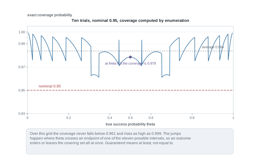
The curve never falls below nominal, averages \(0.984\), and sits above \(0.99\) over wide stretches. The jumps are not noise — there is none here — but the moments when \(\theta\) crosses an endpoint of one of the eleven possible intervals, so an outcome joins or leaves the covering set at once. At \(\theta = 0.5\) the coverage is \(0.979\), matching the hand calculation above: \(1 - 0.02148 = 0.97852\).
Step 5, the degenerate case that makes the argument. Suppose zero of the ten units fail. The lower endpoint is \(0\) by convention and the upper solves \((1 - \theta_U)^{10} = 0.025\), giving \(\theta_U = 1 - 0.025^{1/10} = 0.3085\). The Wald recipe returns \(0 \pm 1.96\sqrt{0 \times 1/10} = (0, 0)\), an interval of zero width asserting the failure probability is exactly zero. Inversion cannot do this, because a whole range of \(\theta\) makes zero failures unsurprising and it keeps every one of them.
What this licenses, and what it does not. You may report that the procedure covers the true failure probability with probability at least \(0.95\) at every \(\theta\) and every sample size, and that every \(\theta_0\) outside \((0.0667, 0.6525)\) would have been rejected by its exact test. You may not report the coverage as \(0.95\): at ten trials it averages \(0.984\), and when methods are compared that difference is the comparison. Nor may you conclude much from three failures in ten units — an interval from \(0.067\) to \(0.653\) fits a very reliable process and a badly broken one alike.
The misreading to avoid
The misreading is one confident sentence: “the interval is \((22.294, 26.906)\), so there is a \(95\) percent probability that \(\mu\) lies between \(22.294\) and \(26.906\) — and since the interval is exact, that probability is exact too.” The second clause makes matters worse: exactness is a property of long-run behaviour, and the sentence has left the procedure behind.
Take the arithmetic first. After the data are observed, \(22.294\) and \(26.906\) are numbers and \(\mu\) is a number, so \(22.294 < \mu < 26.906\) is true or false and its probability under \(P_\mu\) is one or zero. The \(0.95\) attached to the random set \(C(X)\) before the data arrived. Nothing here converts it into a probability about \(\mu\); that needs a prior, and produces a posterior credible set, which Week 14 treats and which is not what was computed above.
The deeper objection is that the long-run figure need not describe your particular data. Let \(X_1, X_2\) be independent and uniform on \((\theta - 1/2, \theta + 1/2)\), and report \(C(X) = [\min(X_1, X_2), \max(X_1, X_2)]\). Writing \(X_i = \theta + U_i\) with \(U_i\) uniform on \((-1/2, 1/2)\), the interval covers \(\theta\) exactly when \(U_1\) and \(U_2\) have opposite signs, which has probability \(1/2\): a genuine \(50\) percent confidence interval whose coverage statement is exactly true.
Now look at the data. Since \(|X_i - \theta| \le 1/2\) always, you know \(\max - 1/2 \le \theta \le \min + 1/2\). If the observed spread \(R = |X_1 - X_2|\) is at least \(1/2\) then \(\max - 1/2 \ge \min\) and \(\min + 1/2 \le \max\), so \(\theta\) lies inside the reported interval with certainty; and \(R \ge 1/2\) happens with probability \(1/4\), since \(R\) has density \(2(1-r)\) on \((0,1)\). Conditionally on \(R = r\) with \(r < 1/2\), the smaller of \(U_1, U_2\) is uniform on an interval of length \(1 - r\) and the interval covers exactly when that minimum lands in a stretch of length \(r\), so the conditional coverage is \(r/(1-r)\), near zero when the observations nearly coincide. The average is honest, \(\int_0^{1/2} \frac{r}{1-r} 2(1-r)\, dr + \int_{1/2}^1 2(1-r)\, dr = 1/4 + 1/4 = 1/2\), but half the time you should be far more confident than \(50\) percent and half the time far less.
Two smaller misreadings travel with the large one. The first is that “conservative” means “careful”: it means actual coverage exceeding nominal, and the price is width, a weaker conclusion than the study paid for. The second is that an interval and a test can disagree on the same data. Two dual procedures cannot. If your software’s interval excludes a value its test does not reject, the two are not dual — they are computed on different scales or from different approximations, which is exactly the Wald behaviour Week 5 dissects.
Practice on your own
These are for self-checking, best attempted before the calibration lab rather than after.
- One-sided inversion. With \(X_1, \dots, X_n\) independent \(N(\mu, \sigma_0^2)\) and \(\sigma_0\) known, invert the level-\(\alpha\) tests of \(H_0 : \mu = \mu_0\) against \(H_1 : \mu > \mu_0\). Show the set is a half-line, state its coverage, and say why the one-sided and two-sided procedures give different endpoints at the same \(\alpha\).
- Optimality transfers. Prove \(P_\theta\{\theta' \in C(X)\} = 1 - \beta_{\theta'}(\theta)\) from the definitions, then argue that inverting uniformly most powerful one-sided tests minimizes the covering probability of every false value.
- Equal tails are not shortest. For the exponential model above, search numerically over pairs \((q_1, q_2)\) with \(P(q_1 \le \chi^2_{20} \le q_2) = 0.95\) for the pair minimizing the width of the interval for \(\lambda\). Report how much narrower it is, and explain why the gain is small.
- Coverage by enumeration. Compute the exact coverage of the exact, Wald, and score intervals for \(n = 25\) over a grid of \(\theta\), starting from the code below. Report the minimum and average of each, and say which you would use for a study reporting a small proportion.
- Where inversion misbehaves. Construct a data value for which a set built by inverting a sensible test family is empty or unbounded, and explain why that does not violate the coverage guarantee. Fieller’s ratio problem is one route; a discrete conditional test is another.
exact_ends <- function(n, k) {
  c(if (k == 0) 0 else qbeta(0.025, k, n - k + 1),
    if (k == n) 1 else qbeta(0.975, k + 1, n - k))
}
cover_at <- function(n, theta, method) {
  ends <- vapply(0:n, function(k) method(n, k), numeric(2))
  sum(dbinom(0:n, n, theta)[ends[1, ] <= theta & theta <= ends[2, ]])
}
cover_at(10, 0.5, exact_ends)                 # 0.9785
mean(sapply(seq(0.05, 0.95, by = 0.001), cover_at, n = 25, method = exact_ends))
Where to read more
- The duality argument and pivotal-quantity constructions are developed in the lecture materials for MIT OpenCourseWare 18.655 Mathematical Statistics.
- A slower, example-first treatment of intervals for means and proportions is in Penn State STAT 415.
- The optional Hogg, McKean, and Craig alignment for this week is Chapter 4.1 through 4.6. That book is optional and is never required to be purchased.
- The enumeration above uses only base R and the
statspackage; see The R Project for Statistical Computing and Quarto. - Course pages: the syllabus, the schedule, the resources overview, and the notes overview. Reread the monotone likelihood ratio material in Week 3 beside step 2 of the second worked example.
Where this goes next
Every exact procedure here depended on special structure: a location-scale family that produced a pivot, or a discrete model small enough to enumerate. Week 5 asks what to do when neither is available, and answers with three statistics built from the log-likelihood alone — likelihood ratio, score, and Wald. Two appear above in disguise: the score interval inverts the score test, and the Wald interval whose coverage sank to \(0.639\) inverts an approximate pivot, which is precisely why its coverage is approximate.
Carry two habits forward. Ask what family of tests an interval inverts, because that names its assumptions; and ask what its actual coverage is at the sample size you have, because a nominal level is a request rather than a report. If a step went past you, repair the duality proof first and the coverage identity second, then use the notes overview for Week 2’s power function or Week 3’s monotone likelihood ratio argument.