Week 5 — Likelihood-ratio, score, and Wald procedures

Where this week starts

The last three weeks gave you exact machinery and told you exactly when it applies. The Neyman-Pearson lemma settles a simple null against a simple alternative. Karlin-Rubin extends that to a one-sided family, but only when the likelihood ratio is monotone in one statistic. Week 4 turned a family of level-\(\alpha\) tests into a confidence set by inversion, and that argument needed a pivot or an exactly computable acceptance region. Every one of those results is a gift with a receipt: it holds because the model has a particular structure, and it stops holding the moment the structure does.

Most models a graduate student actually meets have no such structure. A logistic regression with four covariates, a gamma model with unknown shape and rate, a multinomial with a constraint across cells: none of these hands you a monotone likelihood ratio in a single statistic or a pivot. What all of them do hand you is a log-likelihood function. This week’s question is what you can extract from that function alone, without exact optimality, and what the extraction costs. What the week delivers is three statistics — likelihood ratio, score, and Wald — that read three different features off the same curve, share one limiting distribution, and disagree with each other at every finite sample size.

Keep straight from the start which model each construction has to fit: the likelihood-ratio statistic needs both fits, the score statistic needs only the null fit, and the Wald statistic needs only the unrestricted fit, which is why software prints it by default. What should feel different by the end is your reaction to the phrase “the chi-square test”. There is no such single thing, only three statistics with a common limit under stated conditions, whose agreement is an asymptotic statement rather than a property of your data set. You should also leave able to check the approximation instead of trusting it: in a discrete model the exact size can often be computed by enumeration, and where it cannot, a short simulation settles it.

Why this matters beyond the theorem

Here is the stake, in the smallest honest example this page can offer. Twelve independent trials produce three successes, and someone asks whether the underlying success probability is one half. The Wald statistic is 4.00, above the usual cutoff of 3.84, so default software output reports a significant departure at level 0.05. The likelihood-ratio and score statistics, on the same twelve observations against the same null, are 3.14 and 3.00, and neither crosses. The exact binomial calculation, which needs no approximation at all, gives a two-sided p-value of 0.146. One of these procedures has produced a conclusion the data do not support, and no care in the write-up repairs a statistic that was miscalibrated before the sentence was written.

The reverse failure is less often noticed. When the null value sits on the boundary of the parameter space — a variance component that cannot be negative, a mixing weight that cannot fall below zero — the chi-square reference errs in the conservative direction, and a procedure that quietly halves its own size throws away power the study paid for. Both failures have one source: a limiting distribution invoked without checking the conditions that produce it.

What you will be able to do

• Derive the likelihood-ratio, score, and Wald statistics from the log-likelihood of a stated model, and say which fit each one requires.
• State the conditions under which the chi-square limit holds, give the degrees of freedom as the difference in dimension between two nested models, and identify which condition fails in a problem you are handed.
• Compute all three statistics on a small data set and explain their ordering from the shape of the log-likelihood rather than from a rule of thumb.
• Verify that the likelihood-ratio statistic and the expected-information score statistic are invariant under a smooth invertible reparameterization, and demonstrate that the Wald statistic is not.
• Diagnose a null on the boundary of the parameter space, give the correct limiting law, and supply the cutoff that restores the intended level.
• Design an exact or simulated size study that decides whether the chi-square approximation is trustworthy at the sample size you actually have.

Terms and notation worth fixing

Symbol	What it means on this page
\(\ell(\theta)\)	Log-likelihood of the whole sample, \(\sum_{i=1}^n \log f(x_i; \theta)\), with additive constants dropped freely
\(U(\theta)\)	Score, the first derivative \(\ell'(\theta)\); a random function of the data
\(I_1(\theta)\), \(I_n(\theta)\)	Fisher information for one observation and for the sample, \(I_n(\theta) = n I_1(\theta)\)
\(J(\theta)\)	Observed information, \(-\ell''(\theta)\); a random quantity, not an expectation
\(\hat\theta\), \(\hat\theta_0\)	Maximizer of \(\ell\) over \(\Theta\), and over the null set \(\Theta_0\)
\(\Lambda\), \(S\), \(W\)	The likelihood-ratio, score, and Wald statistics defined below
\(q\)	Degrees of freedom, equal to \(\dim \Theta - \dim \Theta_0\)
\(\chi^2_q\)	Chi-square law on \(q\) degrees of freedom; its 0.95 quantile at \(q = 1\) is 3.84

Three statistics from one log-likelihood

Fix a model \(\{f(\cdot; \theta) : \theta \in \Theta\}\) with \(\Theta\) an open subset of \(\mathbb{R}^p\), and a null set \(\Theta_0 \subset \Theta\) of dimension \(p - q\). All three statistics are built from the single function \(\ell\), and the cleanest way to hold them in mind is geometric: each is twice a vertical drop on a curve, and the three curves differ.

The same log-likelihood produces three different statistics, each twice a vertical drop.

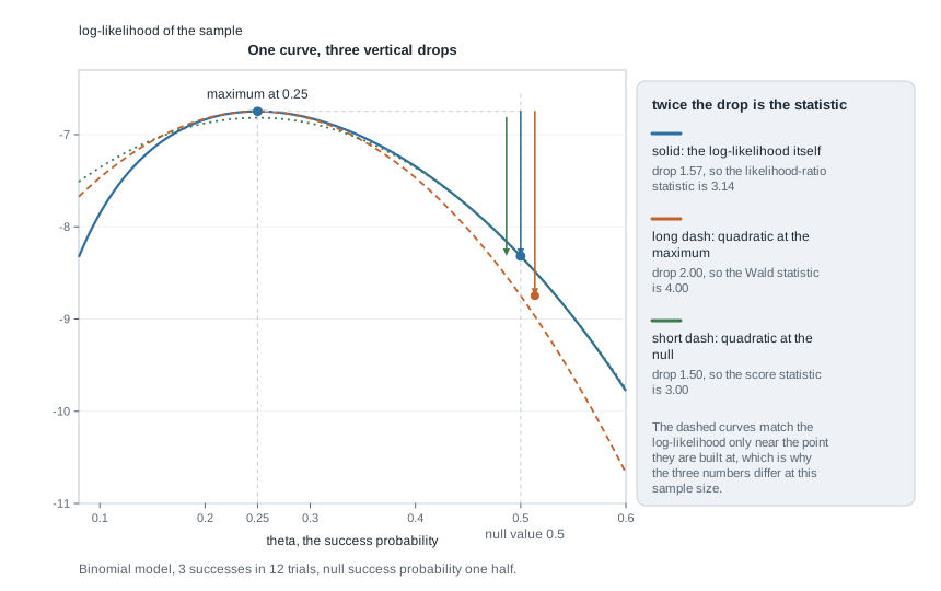
The solid curve is a real log-likelihood, for three successes in twelve trials. The long-dashed curve matches it in value, slope, and curvature at the maximum; the short-dashed curve matches it in value and slope at the null value, with curvature from the expected information there. Twice the drop to the null value is a statistic in each case, and because the three curves are different functions, the three numbers are different numbers.

Building the three statistics

Take the scalar case first, with \(\Theta \subseteq \mathbb{R}\) and the simple null \(H_0 : \theta = \theta_0\) for an interior point \(\theta_0\). The three statistics are

\[ \Lambda = 2\{\ell(\hat\theta) - \ell(\theta_0)\}, \qquad S = \frac{U(\theta_0)^2}{I_n(\theta_0)}, \qquad W = (\hat\theta - \theta_0)^2 \, I_n(\hat\theta). \]

Read them one at a time. \(\Lambda\) compares the height of the log-likelihood at its maximum with its height at the null value, and is large when the null value explains the data poorly relative to the best available. \(S\) asks instead whether the log-likelihood is still climbing at the null value: \(U(\theta_0)\) is the slope there, and dividing by \(I_n(\theta_0)\) standardizes it, since \(U(\theta_0)\) has mean zero and variance \(I_n(\theta_0)\) under the null. \(W\) asks how far the maximizer sits from the null value, in units set by the curvature at the maximizer; a flat log-likelihood makes \(I_n(\hat\theta)\) small and forgives a large distance, a sharply peaked one does not.

For a composite null the same three ideas survive. The likelihood-ratio statistic becomes \(\Lambda = 2\{\ell(\hat\theta) - \ell(\hat\theta_0)\}\), twice the drop from the unrestricted maximum to the best fit inside \(\Theta_0\). The score statistic evaluates the full gradient at the restricted fit \(\hat\theta_0\) and standardizes it by the inverse information matrix, producing a quadratic form. The Wald statistic writes the null as \(g(\theta) = 0\) for a smooth \(g : \Theta \to \mathbb{R}^q\) whose derivative matrix has full rank \(q\), and standardizes \(g(\hat\theta)\) by its delta-method variance. Note the practical consequence: the score statistic never requires the unrestricted fit and the Wald statistic never requires the restricted fit, so when one of the two fits is hard, that fact alone can decide the choice.

Two versions of the Wald statistic circulate, one using expected information \(I_n(\hat\theta)\) and one using observed information \(J(\hat\theta)\). They differ in general, but agree at the maximizer in a full-rank exponential family, for two reasons acting in turn. In the canonical parameterization the second derivative of the log-likelihood does not involve the data at all, so observed and expected information are identically equal there, at every parameter value and not merely at the maximizer. Under a smooth reparameterization a difference between them reappears, but the term carrying it also carries a factor of the score, which vanishes at the maximizer; that transports the equality to any parameterization at that point, and nowhere else in general. That is why the distinction never surfaces in the binomial and Poisson examples below; in a curved or misspecified model it matters, and the observed-information version is usually better behaved.

The regularity that licenses the chi-square limit

Wilks’ theorem is the reason all three statistics get compared with the same reference. State it with its conditions, because the conditions are what this week is really about. Let \(X_1, \dots, X_n\) be independent and identically distributed from \(f(\cdot; \theta)\), and suppose:

1. the support \(\{x : f(x; \theta) > 0\}\) does not depend on \(\theta\);
2. the model is identifiable, so distinct parameter values give distinct distributions, and the maximizer is consistent for the true value — identifiability alone does not deliver consistency, which needs a uniform law of large numbers or a compactness argument on top of it;
3. the true \(\theta\) lies in the interior of \(\Theta\), and under the null it also lies in the relative interior of \(\Theta_0\), which is a smooth submanifold of dimension \(p - q\);
4. \(\ell\) is three times continuously differentiable in a neighbourhood of the true value, with the third derivative bounded by a function whose expectation is finite;
5. differentiation under the integral sign is valid twice, so that \(E_\theta U(\theta) = 0\) and \(\operatorname{Var}_\theta U(\theta) = I_n(\theta)\);
6. \(I_1(\theta)\) is finite, positive definite, and continuous at the true value.

Then, under \(H_0\), each of \(\Lambda\), \(S\), and \(W\) converges in distribution to \(\chi^2_q\), and any two of them differ by a quantity that converges to zero in probability.

The derivation in the scalar case is short enough to keep in your head, and it shows exactly where each condition enters. Expand the score about \(\theta_0\) and evaluate at the maximizer, where \(U(\hat\theta) = 0\); this step already uses condition 3, since a maximizer on the boundary need not have zero derivative. Writing \(\tilde\theta\) for a point between \(\hat\theta\) and \(\theta_0\),

\[ 0 = U(\hat\theta) = U(\theta_0) + \ell''(\tilde\theta)(\hat\theta - \theta_0) \quad \Longrightarrow \quad \sqrt{n}(\hat\theta - \theta_0) = \frac{n^{-1/2} U(\theta_0)}{-n^{-1}\ell''(\tilde\theta)} . \]

Condition 5 makes \(U(\theta_0)\) a sum of independent mean-zero terms with variance \(I_1(\theta_0)\) each, so the numerator converges in distribution to \(N(0, I_1(\theta_0))\) by the central limit theorem. Conditions 4 and 6 make the denominator converge in probability to \(I_1(\theta_0)\) by the law of large numbers together with consistency of \(\hat\theta\). Slutsky’s theorem then gives \(\sqrt{n}(\hat\theta - \theta_0) \to N(0, I_1(\theta_0)^{-1})\), from which \(W \to \chi^2_1\) follows immediately, and the same normal limit for \(n^{-1/2}U(\theta_0)\) gives \(S \to \chi^2_1\) directly.

For \(\Lambda\), expand \(\ell\) about \(\hat\theta\) instead, using \(U(\hat\theta) = 0\) again:

\[ \ell(\theta_0) = \ell(\hat\theta) + \tfrac{1}{2}\ell''(\bar\theta)(\theta_0 - \hat\theta)^2 \quad \Longrightarrow \quad \Lambda = J(\bar\theta)\,(\hat\theta - \theta_0)^2 , \]

for some \(\bar\theta\) between the two. Since \(J(\bar\theta)/n \to I_1(\theta_0)\) in probability, the right-hand side differs from \(W\) only in which consistent estimate of the information it uses, so the two are asymptotically equivalent, and the chi-square limit transfers. Notice what the identity actually says at finite \(n\): \(\Lambda\) uses the average curvature between \(\hat\theta\) and \(\theta_0\), while \(W\) uses the curvature at \(\hat\theta\) alone. When the log-likelihood is asymmetric those are different numbers, and the disagreement you will compute below is exactly this difference.

The degrees of freedom are the most commonly mis-stated part of the theorem. They equal \(\dim \Theta - \dim \Theta_0\), the number of free parameters the null removes, not the number of parameters in either model: testing two of five regression coefficients gives \(q = 2\), testing whether a single proportion equals one half gives \(q = 1\), and testing homogeneity of five proportions gives \(q = 4\), because the null leaves one free parameter where the full model had five.

Condition 1 is not decoration. Take \(X_1, \dots, X_n\) uniform on \((0, \theta)\) and test \(H_0 : \theta = \theta_0\). Here \(\ell(\theta) = -n\log\theta\) for \(\theta \ge X_{(n)}\) and minus infinity below, so \(\hat\theta = X_{(n)}\) and \(\Lambda = 2n\log(\theta_0 / X_{(n)})\). Under the null \(X_{(n)}/\theta_0\) has the distribution of \(V^{1/n}\) for \(V\) uniform on \((0,1)\), so \(\Lambda = -2\log V\), which is exactly \(\chi^2_2\) for every \(n\). Referring \(\Lambda\) to \(\chi^2_1\) would give a test of size \(P(\chi^2_2 > 3.84) = e^{-1.92} = 0.146\) instead of 0.05, and no increase in sample size repairs it, because the statement is exact at every \(n\). The support moves with the parameter, the score identity in condition 5 fails, and the theorem simply does not apply.

Where the three tests part company

Asymptotic equivalence says the three statistics agree in the limit. It says nothing about the size of the disagreement at your sample size, and nothing about which of the three is closer to right when they disagree. In a discrete model those questions can be settled exactly rather than approximately: enumerate every outcome, compute each statistic, and add the null probabilities of the outcomes each test rejects. That is a size calculation with no Monte Carlo error in it at all.

The figure below does this for a binomial proportion, testing \(H_0 : \theta = 0.3\) against \(H_1 : \theta \ne 0.3\) when 0.3 is in fact the true success probability, across sample sizes 10 through 60, at nominal level 0.05. Two features matter. The sawtooth is discreteness: the achievable sizes jump as the critical count moves by one, the same conservatism Week 4 met in exact binomial intervals. The systematic vertical offset is approximation error, and it does not average away.

Exact size of the three tests against sample size, at nominal level 0.05.

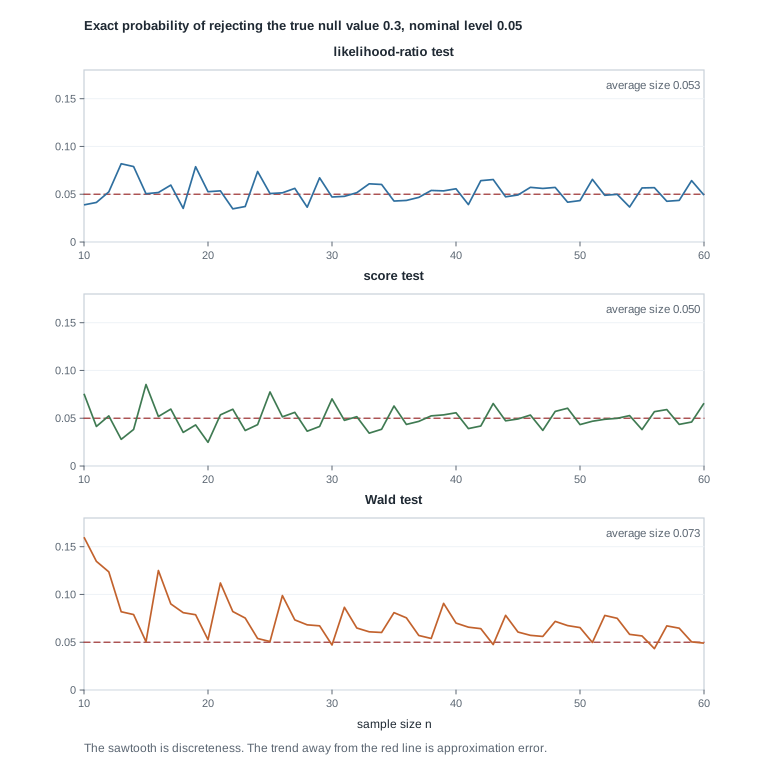
Averaged over these fifty-one sample sizes the exact size is 0.053 for the likelihood-ratio test, 0.050 for the score test, and 0.073 for the Wald test. The Wald test is not merely noisier; it rejects true nulls more often than it claims to, and it does so consistently. At \(n = 10\) its exact size is 0.16, more than three times the nominal level.

Parameterization and what is invariant

The Wald statistic has a second and more troubling property: it depends on the scale you chose to write the parameter in. Let \(\psi = g(\theta)\) for a smooth, strictly increasing \(g\), so that \(H_0 : \theta = \theta_0\) and \(H_0 : \psi = g(\theta_0)\) are the same hypothesis about the same distribution. The likelihood-ratio statistic cannot change: \(\Lambda\) depends on the model only through the attained maxima of the likelihood over \(\Theta\) and over \(\Theta_0\), and relabelling the points of a set does not change the supremum of a function over it. So \(\Lambda\) is exactly invariant, at every sample size, with no appeal to asymptotics.

The score statistic with expected information is invariant too, and the computation is worth doing once. With \(\theta = h(\psi)\) the chain rule gives \(U_\psi(\psi_0) = U_\theta(\theta_0) h'(\psi_0)\), while \(I_\psi(\psi_0) = E\{U_\psi^2\} = I_\theta(\theta_0) h'(\psi_0)^2\) exactly. The factors \(h'(\psi_0)^2\) cancel in the ratio, so \(S\) is unchanged. The same cancellation fails for observed information, because \(J_\psi = J_\theta h'^2 - U_\theta h''\), and that second term vanishes only where the score is zero. So a score test built on observed information is not exactly invariant, and if you report one you should say which information you used.

The Wald statistic has no such protection. It measures a squared distance on whichever scale you wrote down, standardized by a curvature computed on that same scale, and a nonlinear reparameterization changes both in ways that do not cancel. The second worked example takes one hypothesis through two scales and reaches two conclusions from the same twelve observations. No rule makes one scale canonical, which is the strongest practical argument for reporting a likelihood-ratio result whenever you can compute both fits.

Boundary nulls and the failure of the chi-square limit

Condition 3 fails whenever the null value sits on the edge of the parameter space, which happens far more often than the phrase “boundary case” suggests: a variance component that must be non-negative, a correlation at one, a mixture weight at zero. The repair is not hard, but the naive procedure is wrong every time. Take the cleanest instance. Let \(X_1, \dots, X_n\) be independent \(N(\mu, 1)\) with the parameter space \(\Theta = \{\mu \ge 0\}\), and test \(H_0 : \mu = 0\), so that \(\Theta_0 = \{0\}\) and \(\mu = 0\) is a boundary point of \(\Theta\) rather than an interior one. Maximizing \(\ell\) over \(\Theta\) gives \(\hat\mu = \max(\bar X, 0)\), and substituting yields \(\Lambda = n\bar X^2\) when \(\bar X > 0\) and \(\Lambda = 0\) otherwise. Under the null \(\sqrt{n}\bar X\) is standard normal, so \(\Lambda\) equals zero with probability one half; and conditionally on \(\bar X > 0\) the quantity \(n\bar X^2\) has exactly the \(\chi^2_1\) law, because a standard normal conditioned to be positive has the same law of its square as an unconditioned one. The null distribution is therefore the mixture \(\tfrac{1}{2}\delta_0 + \tfrac{1}{2}\chi^2_1\), sometimes written \(\bar\chi^2\), and not \(\chi^2_1\).

A boundary null halves every tail probability, so the usual cutoff halves the size.

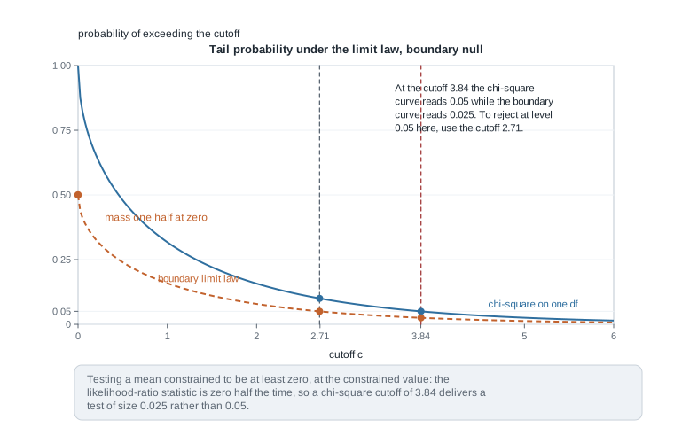
The consequence is quantitative and easy to state. Referring \(\Lambda\) to \(\chi^2_1\) and rejecting above 3.84 produces a test of size \(\tfrac{1}{2}(0.05) = 0.025\), so the procedure is valid but wastes half its level. To get a test of size 0.05 you need the cutoff \(c\) with \(\tfrac{1}{2}P(\chi^2_1 > c) = 0.05\), which is the 0.90 quantile of \(\chi^2_1\), namely 2.71. That one substitution recovers the power the naive procedure discards. Two warnings before you generalize. The one-half weight comes from one parameter tested at one boundary; several constrained parameters produce mixtures over several degrees of freedom with weights that are not one half. And the Wald statistic fares worse here than the likelihood ratio, because the estimate piles up at the boundary and the quadratic expansion behind \(W\) has no interior maximum to expand around.

Worked example — three statistics for a binomial proportion

The model and the question. A screening procedure in a clinical laboratory is applied to twelve independent specimens, and three of them are flagged. Model the count as \(X \sim \text{Binomial}(12, \theta)\) and test \(H_0 : \theta = 0.5\) against \(H_1 : \theta \ne 0.5\) at level 0.05. Check the conditions first: the support \(\{0, 1, \dots, 12\}\) does not depend on \(\theta\); the model is identifiable; \(\theta_0 = 0.5\) is interior to \((0,1)\); \(\ell\) is smooth there; and \(I_n(\theta) = n/\{\theta(1-\theta)\}\) is finite and positive. Wilks’ theorem applies, with \(q = 1 - 0 = 1\). Nothing in the theorem says \(n = 12\) is large enough for it to be useful, and that gap is the entire point of the example.

Step 1, the log-likelihood and the maximizer. Dropping the binomial coefficient, \(\ell(\theta) = 3\log\theta + 9\log(1-\theta)\). Setting the derivative to zero gives \(\hat\theta = 3/12 = 0.25\).

Step 2, the score and the information. \(U(\theta) = 3/\theta - 9/(1-\theta)\), so \(U(0.5) = 6 - 18 = -12\). The information is \(I_n(\theta) = 12/\{\theta(1-\theta)\}\), giving \(I_n(0.5) = 12/0.25 = 48\) and \(I_n(0.25) = 12/0.1875 = 64\).

Step 3, the likelihood-ratio statistic.

\[ \Lambda = 2\{\ell(0.25) - \ell(0.5)\} = 2\left\{3\log\frac{0.25}{0.5} + 9\log\frac{0.75}{0.5}\right\} = 2\{3(-0.69315) + 9(0.40546)\} = 2(1.56973) = 3.139 . \]

Step 4, the score statistic. \(S = U(0.5)^2 / I_n(0.5) = 144/48 = 3.000\). Equivalently \(S = n(\hat\theta - \theta_0)^2/\{\theta_0(1-\theta_0)\} = 12(0.0625)/0.25\), which is the familiar normal-approximation statistic with the null value in the standard error.

Step 5, the Wald statistic. \(W = (0.25 - 0.5)^2 \times 64 = 0.0625 \times 64 = 4.000\). Here the standard error uses \(\hat\theta\) rather than \(\theta_0\), and because \(0.25 \times 0.75\) is smaller than \(0.5 \times 0.5\), the denominator shrinks and the statistic grows.

Step 6, referring each to \(\chi^2_1\). The 0.95 quantile is 3.84. The approximate p-values are 0.076 for \(\Lambda\), 0.083 for \(S\), and 0.046 for \(W\). The Wald test rejects at level 0.05; the other two do not.

Step 7, the exact calculation. Because the null distribution is \(\text{Binomial}(12, 0.5)\) and symmetric, the two-sided exact p-value is \(2P(X \le 3) = 2(1 + 12 + 66 + 220)/4096 = 598/4096 = 0.146\). All three approximations understate the tail, and the Wald approximation understates it by a factor of three.

Four p-values for the same outcome: three approximations and the exact calculation.

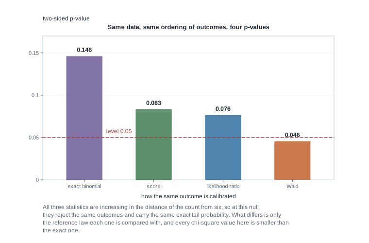
What this licenses, and what it does not. All three statistics here are increasing functions of \(|x - 6|\), so at this null they order the sample space identically and attach the same exact tail probability to this outcome. What differs is only the reference distribution each is compared with: the quality of an approximation, not a disagreement about evidence. You may defend the conclusion that twelve observations are consistent with a success probability of one half. You may not defend the Wald rejection, which is an artefact of fitting a quadratic to an asymmetric log-likelihood at a sample size where the asymmetry is large — in the figure at the head of this page, that quadratic sits below the true curve at 0.5, so the drop it reports is too big.

A short block of R reproduces the numbers above.

three_stats <- function(n, x, p0) {          # valid for 0 < x < n
  hat <- x / n
  c(lr    = 2 * (x * log(hat / p0) + (n - x) * log((1 - hat) / (1 - p0))),
    score = n * (hat - p0)^2 / (p0 * (1 - p0)),
    wald  = n * (hat - p0)^2 / (hat * (1 - hat)))
}
stat <- three_stats(12, 3, 0.5)
round(stat, 3)
round(pchisq(stat, df = 1, lower.tail = FALSE), 3)
round(binom.test(3, 12, p = 0.5)$p.value, 3)

The same reasoning, transferred

Now change the model and keep the structure. Ten counts from a reliability test are modelled as \(X_i \sim \text{Poisson}(\lambda)\), their total is \(\sum x_i = 6\), and the null is \(H_0 : \lambda = 1\). Dropping constants, \(\ell(\lambda) = -10\lambda + 6\log\lambda\), so \(\hat\lambda = \bar{x} = 0.6\). The score is \(U(\lambda) = 6/\lambda - 10\), giving \(U(1) = -4\), and the information is \(I_n(\lambda) = 10/\lambda\), giving \(I_n(1) = 10\) and \(I_n(0.6) = 16.67\). Then

\[ \Lambda = 2\{(-6 + 6\log 0.6) - (-10)\} = 1.870, \qquad S = \frac{16}{10} = 1.600, \qquad W = (0.4)^2 \times 16.67 = 2.667 . \]

The approximate p-values are 0.171, 0.206, and 0.102, and none of the three rejects at level 0.05. For a rough exact comparison, \(\sum X_i\) is Poisson with mean 10 under the null, and twice the lower tail \(2P(\sum X_i \le 6) = 0.260\) — one of several conventions for a two-sided p-value in a skewed discrete model — again exceeds all three approximations.

What stayed the same: the three constructions, the single degree of freedom, the ordering \(S < \Lambda < W\) — common when the estimate falls where the log-likelihood is flatter than the quadratic at the null, though no theorem guarantees it — and the direction of the error, every chi-square p-value being smaller than the exact one. What changed: the information function, \(n/\lambda\) here rather than \(n/\{\theta(1-\theta)\}\), and the geometry of the parameter space, since \(\lambda\) is bounded below by zero. That last change is not cosmetic. Had the total been \(\sum x_i = 0\), the maximizer would sit at the boundary point \(\hat\lambda = 0\) and the Wald statistic would be undefined, since \(I_n(0)\) does not exist. The likelihood-ratio statistic is still computable, at \(2n\lambda_0\), but condition 3 has failed and \(\chi^2_1\) is no longer its reference.

Second worked example — the same hypothesis on two scales

The model and the question. Keep the data of the first example — three successes in twelve trials — and keep the hypothesis. Write it twice. On the probability scale it is \(H_0 : \theta = 0.5\). On the log-odds scale, with \(\psi = \log\{\theta/(1-\theta)\}\), it is \(H_0 : \psi = 0\). These are the same statement about the same distribution; the map is smooth and strictly increasing, so nothing statistical has changed. The question is whether the Wald test notices.

Step 1, the probability scale. From the first example, \(\hat\theta = 0.25\) with estimated standard error \(\sqrt{\hat\theta(1-\hat\theta)/n} = \sqrt{0.1875/12} = 0.125\), so \(W_\theta = (0.25 - 0.5)^2/(0.125)^2 = 0.0625/0.015625 = 4.000\), with approximate p-value 0.046. The interval that inverts this test is \(0.25 \pm 1.96(0.125)\), that is \((0.005, 0.495)\), and it excludes 0.5 — the same conclusion as the test, as Week 4’s duality requires.

Step 2, the log-odds scale. Here \(\hat\psi = \log(0.25/0.75) = -1.0986\). The information for \(\psi\) is \(I_n(\psi) = n\theta(1-\theta)\), so at the estimate \(I_n(\hat\psi) = 12(0.25)(0.75) = 2.25\) and the standard error is \(1/\sqrt{2.25} = 0.6667\). The delta method agrees: \(0.125 / \{0.25 \times 0.75\} = 0.6667\). Then

\[ W_\psi = \frac{(-1.0986)^2}{(0.6667)^2} = \frac{1.207}{0.4444} = 2.716 , \]

with approximate p-value 0.099. The interval is \(-1.0986 \pm 1.96(0.6667) = (-2.405, 0.208)\), and transforming back through \(\theta = 1/(1 + e^{-\psi})\) gives \((0.083, 0.552)\), which contains 0.5.

The same Wald procedure on two scales, both drawn on the probability axis.

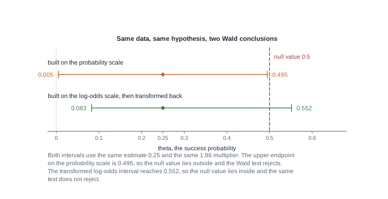
Step 3, what the other two statistics do. On the log-odds scale \(\ell(\psi) = x\psi - n\log(1 + e^{\psi})\), so \(U_\psi(0) = 3 - 12(0.5) = -3\) and \(I_n(\psi_0) = 12(0.5)(0.5) = 3\), giving \(S = 9/3 = 3.000\) — the same 3.000 computed on the probability scale, exactly as the invariance argument promised. The likelihood-ratio statistic is 3.139 on both scales, because the maximized likelihoods being compared are the same two numbers.

Step 4, what it licenses. The same data, the same hypothesis, and the same procedure name have produced p-values of 0.046 and 0.099, one on each side of the conventional level. Neither is the more correct application of the Wald recipe; both are legitimate Wald tests, and that is the complaint. The log-odds version behaves better here because the log-likelihood is closer to quadratic in \(\psi\) than in \(\theta\) — \(\psi\) is the canonical parameter of the family — so the approximation the Wald statistic leans on is under less strain. You learn that by studying the model, not by reading output, and nothing in the Wald construction tells you which scale you are on. The likelihood-ratio and score statistics needed no such judgement.

The misreading to avoid

The misreading is a sentence that sounds like sophistication: “the three tests are asymptotically equivalent, so it doesn’t matter which one I report — I’ll use whichever my software prints.” Every clause of that is defensible except the inference joining them.

Asymptotic equivalence is a precise claim, with a fixed model, a fixed null, all six regularity conditions holding, and \(n \to \infty\): the differences among \(\Lambda\), \(S\), and \(W\) converge to zero in probability. It does not say the differences are small at your \(n\), and it supplies no bound at any finite \(n\). On twelve observations this page produced 3.139, 3.000, and 4.000 for one hypothesis, p-values of 0.076, 0.083, and 0.046 against an exact 0.146, and one rejection out of three. Nothing there violates the theorem; the limit is simply not the sample size in front of you.

The claim also assumes the conditions hold, and two of this week’s examples are settings where the premise fails outright: at a boundary null the likelihood-ratio statistic converges to a mixture while the Wald statistic degenerates, and with a support that moves with the parameter the likelihood-ratio statistic has an exact \(\chi^2_2\) law that no sample size erodes. The equivalence cannot rescue you in exactly the situations where you need rescuing. Nor is the Wald statistic equivalent to itself: two analysts fitting the identical model to the identical data, one on the probability scale and one on the log-odds scale, reported 0.046 and 0.099 above, and a quantity that changes when you rewrite the parameter is reporting your notation as well as your data.

Two smaller misreadings travel with the big one. The first is that the degrees of freedom count parameters; they count the difference in dimension between two nested models, and if you cannot say which model is nested in which, you cannot yet write down \(q\). The second is that “\(n\) is large” settles the approximation. Large relative to what? For a proportion near a boundary what governs the approximation is the smaller expected count: a thousand trials with two expected successes is a small-sample problem wearing a large-sample coat.

Practice on your own

These are for self-checking; work them before the calibration lab rather than after.

1. Scaling. Recompute the three statistics for 12 successes in 48 trials against \(H_0 : \theta = 0.5\) — the same estimate \(\hat\theta = 0.25\), four times the data. Predict how each statistic changes before you compute, then compare the three chi-square p-values with the exact two-sided binomial value and describe what improved and what did not.
2. Invariance, done properly. With \(\theta = h(\psi)\) smooth and strictly increasing, prove that \(U_\theta(\theta_0)^2/I_n(\theta_0)\) is unchanged when the problem is rewritten in \(\psi\), then repeat with observed information, identify the extra term, and say when it vanishes.
3. A model where two of the three coincide. For \(X_1, \dots, X_n\) independent exponential with rate \(\lambda\), derive \(\Lambda\), \(S\), and \(W\) for \(H_0 : \lambda = \lambda_0\). Two of the three are identical for every sample; find which, and explain it. Then rewrite the model in terms of the mean \(\mu = 1/\lambda\) and recompute all three. Which of them moved?
4. An exact size study. Adapt the R block above to enumerate all outcomes of a \(\text{Binomial}(n, 0.2)\) experiment and compute the exact size of each of the three tests at nominal level 0.05, for \(n = 20, 40, 80, 160\). Report the three sizes at each \(n\) and say which test you would trust at \(n = 40\) and why.
5. The boundary, by simulation. Simulate \(N(0,1)\) samples of size 40, compute \(\Lambda = n\max(\bar x, 0)^2\) on each, and estimate the probabilities that \(\Lambda\) is exactly zero, exceeds 3.84, and exceeds 2.71. Compare with one half, 0.025, and 0.05, and report the Monte Carlo standard error of each estimate.

set.seed(2027)
n <- 40
lam <- replicate(20000, { xbar <- mean(rnorm(n)); n * max(xbar, 0)^2 })
c(at_zero = mean(lam == 0),
  above_384 = mean(lam > qchisq(0.95, df = 1)),
  above_271 = mean(lam > qchisq(0.90, df = 1)))

Where to read more

• The large-sample likelihood theory behind Wilks’ theorem, at the level this week assumes, is developed in the lecture materials for MIT OpenCourseWare 18.655 Mathematical Statistics; read the asymptotics of maximum likelihood beside the derivation above.
• A slower, example-first treatment of likelihood-ratio testing, if that derivation moved too quickly, is in Penn State STAT 415.
• The optional Hogg, McKean, and Craig alignment for this week is Chapter 6.3 and 6.5, together with Chapter 8.3. That book is optional and is never required to be purchased.
• The computations here use only base R and the stats package; see The R Project for Statistical Computing and Quarto.
• Course pages: the syllabus, the schedule, the resources overview, and the notes overview. The duality argument in Week 4 is worth rereading beside step 1 of the second worked example.

Where this goes next

Everything here assumed the parameter you care about is the only one there is, or that the null pins down all the others. Week 6 removes that assumption. When \(\theta\) splits into an interest parameter and a nuisance parameter, all three statistics need a rule for eliminating what you do not care about — profiling, conditioning, or invariance — and each rule costs something. The profile likelihood behaves like a log-likelihood in the constructions above, but its curvature overstates the precision available, and that overstatement is next week’s central caution.

The other thread continuing next week is comparison. This page showed the three tests disagreeing under a null; local alternatives are the device that lets you compare their power without the comparison collapsing to “all three have power one”. If a step here went past you, repair the score expansion first and the invariance computation second. The notes overview lists the earlier units if you need Week 2’s power function or Week 4’s inversion argument before going on.