Week 13 — Robust inference, influence, and M-estimation

Where this week starts

Every procedure this course has built rests on something being exactly true: the exact tests of Week 4 need the sampling model to be the model, the three statistics of Week 5 need a smooth and correctly specified likelihood, the randomization tests of Week 10 need the randomization to have happened, and the rank procedures of Week 12 need only continuity but buy that by changing what is estimated. This week takes the case none of them addresses head on: the model is nearly right. Most observations behave exactly as it says and a small remainder does not, because a digit was transposed, an instrument drifted, or the tail is heavier than the model admits.

Week 12 left this half-finished. Rank procedures answer “what if I do not know the shape” by keeping only the ordering, which moves the estimand: the rank-sum test targets an exceedance probability, not a mean. Robust inference asks something narrower — keep the target roughly where it was, and make the procedure’s behaviour continuous in the underlying distribution, so a small perturbation of \(F\) produces only a small perturbation of the estimate and its standard error.

The organizing move is to stop treating an estimator as a function of a sample and treat it as a function of a distribution. Once \(\hat\theta = T(F_n)\) is a functional evaluated at the empirical distribution, you can differentiate \(T\) in the direction of a contaminating point mass. That derivative is the influence function, and the rest follows: the asymptotic variance is the integral of its square, the damage one outlier can do is its supremum, and the estimating equation behind it is M-estimation, whose variance under a wrong model is the sandwich. By the end, “is this estimator robust” should have split into three questions — against which neighbourhood, at what cost in efficiency at the clean model, and for which functional.

Why this matters beyond the theorem

Here is the stake, in the smallest example that shows it. A laboratory records ten replicate readings of the same reference specimen, in coded units: \(4, 7, 7, 7, 8, 9, 10, 14, 14, 16\). The sample mean is \(9.6\) and the sample standard deviation \(3.864\), so the standard error is \(3.864 / \sqrt{10} = 1.222\) and the \(95\) per cent \(t\) interval, using the \(0.975\) quantile \(2.262\) of \(t\) on nine degrees of freedom, is \(9.6 \pm 2.262 \times 1.222 = (6.84, 12.36)\). Now suppose the last reading, truly \(16\), is typed as \(61\). The mean becomes \(14.1\), the standard deviation \(16.776\), the standard error \(5.305\), and the interval \(14.1 \pm 12.00 = (2.10, 26.10)\) — over four times wider, and centred where no honest reading of the data puts it.

Nothing in the output announces the problem. The interval got wider, which reads as caution, so the mistake looks like a noisy instrument rather than overconfidence, and any decision calibrated to that precision is calibrated to a fiction produced by one keystroke. The lesson is not that outliers should be hunted and deleted. It is that a procedure whose output can be moved an unbounded distance by one of \(n\) observations has an operating characteristic nobody stated — and that other procedures exist for which this corruption changes nothing at all.

What you will be able to do

• Write an estimator as a statistical functional and compute its influence function as the derivative at a contaminating point mass, stating the differentiability that computation requires.
• Derive the influence functions of the mean and the median at a stated distribution, and read the gross-error sensitivity and the asymptotic variance off them.
• Compute breakdown points for the mean, the trimmed mean, the median, and a Huber estimator with fixed scale, and say what a breakdown point does and does not promise.
• Define an M-estimator by its estimating equation, solve that equation numerically on a small sample, and identify the functional it targets when the assumed model is false.
• Derive the sandwich variance, state the conditions under which it is valid, and explain why it repairs the standard error rather than the estimand.
• Quantify the efficiency surrendered at the clean model in exchange for bounded influence.

Terms and notation worth fixing

Symbol or term	Meaning as used in this course
\(F\), \(F_n\)	the distribution generating the data, and the empirical distribution of \(X_1, \dots, X_n\)
\(T(F)\)	a statistical functional: a number attached to a distribution. The plug-in estimator is \(T(F_n)\)
\(F_\varepsilon = (1 - \varepsilon) F + \varepsilon H\)	a gross-error neighbourhood: a fraction \(\varepsilon\) of the mass replaced by an arbitrary \(H\)
\(\delta_x\)	the distribution putting all its mass at the single value \(x\)
\(\mathrm{IF}(x; T, F)\)	the influence function: the derivative of \(T\) at \(F\) in the direction of \(\delta_x\)
\(\gamma^{*}\)	gross-error sensitivity, \(\sup_x \lvert \mathrm{IF}(x; T, F) \rvert\): the worst first-order damage one observation can do
\(\varepsilon^{*}\)	breakdown point: the largest fraction of the sample that may be replaced arbitrarily while the estimate stays bounded
\(\psi\)	the estimating function. An M-estimator \(\hat\theta\) solves \(\sum_{i=1}^{n} \psi(X_i, \theta) = 0\)
\(A\), \(B\)	the sandwich ingredients \(A = -E_F[\partial \psi / \partial \theta]\) and \(B = E_F[\psi^2]\), both evaluated at the target value

Throughout, \(\theta_0\) means the value the estimating equation targets in the population, \(T(F)\), while \(\overset{d}{\longrightarrow}\) and \(\overset{P}{\longrightarrow}\) mean convergence in distribution and in probability — every limit below is asymptotic and says nothing by itself about \(n = 10\).

Contamination neighbourhoods and the influence function

Robustness is always robustness against a stated set of alternatives, and the standard set is Tukey’s gross-error model. Fix a central model \(F\) — usually a normal — and a contamination fraction \(\varepsilon\), and consider every \(F_\varepsilon = (1 - \varepsilon) F + \varepsilon H\) with \(H\) completely arbitrary; sampling from it is the same as flipping a coin with success probability \(\varepsilon\) per observation and drawing from \(H\) when it lands. A procedure is robust over the neighbourhood if its behaviour degrades gracefully across the whole of it, and two summaries of “gracefully” are worth having: an infinitesimal one from differentiating at \(\varepsilon = 0\), and a global one, the largest \(\varepsilon\) it survives.

From estimators to statistical functionals

A statistical functional is a rule \(T\) carrying a distribution to a number: the mean \(\mu(F) = \int y \, dF(y)\), the median \(m(F) = F^{-1}(1/2)\) (well defined whenever \(F\) is strictly increasing near that quantile), the variance \(\sigma^2(F) = \int (y - \mu(F))^2 \, dF(y)\). Substituting the empirical distribution \(F_n\), which puts mass \(1/n\) at each observed value, recovers \(\bar{X}\) and the sample median — the plug-in principle you met with the bootstrap in Week 11, to a different end.

The functional view earns its keep because it lets you ask something meaningless for a formula in \(x_1, \dots, x_n\): what happens to the output if the input distribution is nudged? It also forces the distinction the week depends on. If the family \(\{F_\theta\}\) contains the truth and \(T(F_\theta) = \theta\) for every \(\theta\), the functional is Fisher consistent and the two notions of target agree. Outside the family \(T(F)\) still exists and the estimator still converges to it, but it is now whatever number the functional assigns to the true \(F\), and calling that “the parameter” is a choice to be defended rather than assumed.

Differentiating a functional at a point mass

Take the contaminating distribution to be a point mass at \(x\), so \(F_\varepsilon = (1 - \varepsilon) F + \varepsilon \delta_x\), and differentiate at zero contamination. The influence function of \(T\) at \(F\) is

\[\mathrm{IF}(x; T, F) = \lim_{\varepsilon \downarrow 0} \frac{T\big((1 - \varepsilon) F + \varepsilon \delta_x\big) - T(F)}{\varepsilon},\]

when the limit exists. Read it as: if a vanishingly small fraction of the population were replaced by copies of \(x\), the functional would move at this rate per unit of contamination. Two consequences make it central. First, \(\int \mathrm{IF}(y; T, F) \, dF(y) = 0\) whenever the derivative is linear in the contaminating direction, since contaminating \(F\) by \(F\) itself changes nothing; the influence function is therefore centred, like a score. Second, the von Mises expansion: under conditions strong enough to make the remainder negligible,

\[\sqrt{n} \, \big(T(F_n) - T(F)\big) = \frac{1}{\sqrt{n}} \sum_{i=1}^{n} \mathrm{IF}(X_i; T, F) + \sqrt{n} \, R_n ,\]

so that if \(\sqrt{n} \, R_n \overset{P}{\longrightarrow} 0\) and \(\int \mathrm{IF}^2 \, dF\) is finite, the central limit theorem gives

\[\sqrt{n} \, \big(T(F_n) - T(F)\big) \overset{d}{\longrightarrow} N\!\left(0, \int \mathrm{IF}(y; T, F)^2 \, dF(y)\right).\]

State the conditions rather than waving at them. Differentiability along point-mass paths — Gateaux differentiability, which is exactly what the display above defines — is not by itself enough to kill the remainder, because \(F_n\) approaches \(F\) along paths that are not of that form. What does the work is differentiability uniformly over the relevant class of directions, Hadamard differentiability, together with a square-integrable influence function. Where that fails, as for the sample maximum, the normal limit does not hold — the boundary case that broke the bootstrap in Week 11, for the same reason.

Gross-error sensitivity and the breakdown point

The influence function is local, so the natural local summary of danger is its supremum, \(\gamma^{*} = \sup_x \lvert \mathrm{IF}(x; T, F) \rvert\). A functional with finite \(\gamma^{*}\) is bias-robust at \(F\): to first order in \(\varepsilon\), no single contaminating value moves it more than \(\varepsilon \gamma^{*}\). The mean, with infinite \(\gamma^{*}\), has no such bound.

Sensitivity says nothing about a contamination fraction that is not small. For that, use the finite-sample replacement breakdown point: the largest fraction \(m/n\) such that, whatever values are substituted for any \(m\) of the \(n\) observations, the estimate stays bounded. The sample mean has breakdown \(0\), since one replaced observation carries it anywhere. The \(\alpha\)-trimmed mean, which discards the fraction \(\alpha\) at each tail before averaging, has breakdown \(\lfloor \alpha n \rfloor / n\), tending to \(\alpha\); the median has \(\lfloor (n-1)/2 \rfloor / n\), tending to \(1/2\). No translation-equivariant estimator beats one half, because at half contamination there is no way to tell which half is the model.

Breakdown fraction of the trimmed mean rises linearly with the amount trimmed, from the sample mean at zero to the median at one half.

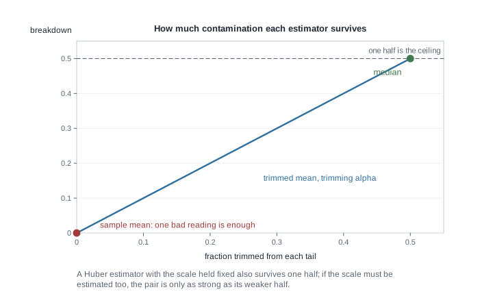
Neither summary implies the other. A high breakdown point is no promise of small bias below breakdown: an estimator can survive \(40\) per cent contamination and still be badly biased at \(10\) per cent. And a bounded influence function promises nothing at \(\varepsilon = 0.3\), being a statement about a derivative at zero.

M-estimators and the sandwich variance

Influence functions diagnose estimators; M-estimation constructs them. Define the estimator implicitly, as the root of an estimating equation, and choose that equation so the influence function comes out bounded. Everything about the result — its target, its influence function, its asymptotic variance, its computation — reads off the estimating function directly.

Estimating equations and the Huber psi function

An M-estimator \(\hat\theta\) is any root of

\[\sum_{i=1}^{n} \psi(X_i, \hat\theta) = 0 ,\]

and when \(\psi = \partial \rho / \partial \theta\) for some \(\rho\), this is the stationarity condition for minimizing \(\sum_i \rho(X_i, \theta)\). Three instances fix the idea: \(\rho(x, \theta) = (x - \theta)^2 / 2\) gives \(\psi(x, \theta) = x - \theta\) and the sample mean; \(\rho(x, \theta) = \lvert x - \theta \rvert\) gives \(\psi(x, \theta) = \mathrm{sign}(x - \theta)\) and the sample median, the equation being solved in the generalized sense of a sign change because \(\psi\) is a step; and \(\rho\) the negative log-likelihood gives \(\psi\) equal to the score, so M-estimation contains Weeks 5 and 6 as a special case.

Huber’s proposal is the compromise between the first two. With a tuning constant \(k > 0\),

\[\rho_k(u) = \tfrac{1}{2} u^2 \quad \text{for } \lvert u \rvert \le k, \qquad \rho_k(u) = k \lvert u \rvert - \tfrac{1}{2} k^2 \quad \text{for } \lvert u \rvert > k ,\]

whose derivative is the clipped identity

\[\psi_k(u) = u \quad \text{for } \lvert u \rvert \le k, \qquad \psi_k(u) = k \, \mathrm{sign}(u) \quad \text{for } \lvert u \rvert > k .\]

The pieces meet so that \(\rho_k\) is continuously differentiable at \(\lvert u \rvert = k\): both one-sided derivatives equal \(k\) and both expressions give \(k^2/2\). Squared error near the centre, absolute error in the tails.

The Huber loss follows the parabola near zero and becomes linear beyond the tuning constant, so its derivative is flat past that point.

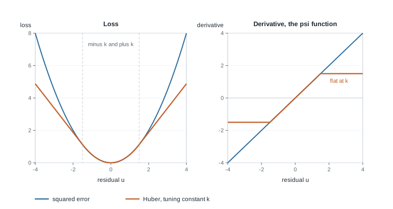
The functional an M-estimator targets is the root \(\theta_0 = T(F)\) of \(\int \psi(y, \theta) \, dF(y) = 0\), assumed unique. Differentiating that relation as before gives every M-estimator’s influence function in one line:

\[\mathrm{IF}(x; T, F) = \frac{\psi(x, \theta_0)}{A}, \qquad A = -\int \frac{\partial \psi}{\partial \theta}(y, \theta_0) \, dF(y) .\]

An M-estimator’s influence function is its own \(\psi\), rescaled: bounded \(\psi\) means bounded influence, and that sentence is the design principle of the whole subject. For the mean, \(\partial \psi / \partial \theta = -1\) gives \(A = 1\) and \(\mathrm{IF}(x) = x - \mu\). For the Huber \(\psi\), \(\psi_k'\) is one on the interior and zero outside, so \(A = P_F(\lvert X - \theta_0 \rvert \le k)\) provided \(F\) puts no mass at \(\theta_0 \pm k\), and \(\gamma^{*} = k / A\), finite for every finite \(k\). When \(\psi\) jumps, read \(A\) off the population function instead of pointwise: for the median \(\partial \psi / \partial \theta\) is zero almost everywhere, which would give \(A = 0\), yet \(\lambda(\theta) = E_F \, \mathrm{sign}(X - \theta) = 1 - 2 F(\theta)\) gives \(A = -\lambda'(m) = 2 f(m)\) and the influence function \(\mathrm{sign}(x - m) / (2 f(m))\) derived from scratch below.

The tuning constant is the price list: small \(k\) approaches the median, large \(k\) the mean. The table reports asymptotic variances of \(\sqrt{n}(\hat\theta - \theta_0)\) with \(\sigma = 1\), computed from \(E[\psi^2] / (E[\psi'])^2\) at each distribution; the clean-normal entries for the mean and median are the exact values \(1\) and \(\pi/2\), the rest numerical evaluations of the same integrals.

Estimator	at the exact normal	at \(0.9 \, N(0,1) + 0.1 \, N(0,9)\)
sample mean	\(1.00\)	\(1.80\)
Huber, \(k = 1.345\)	\(1.05\)	\(1.30\)
sample median	\(1.57\)	\(1.80\)

Read the columns together, because either alone misleads. At the clean model the mean wins and the median needs about \(57\) per cent more observations to match it; under ten per cent contamination by a distribution three times as spread out, the mean and median are essentially tied and the Huber estimator beats both. Nothing is uniformly best — the risk-function situation of Week 1, with the neighbourhood playing the part of the parameter space.

The sandwich, its conditions, and what it does not repair

Expand the estimating equation about \(\theta_0\). Writing \(\psi_i(\theta) = \psi(X_i, \theta)\) and assuming \(\hat\theta \overset{P}{\longrightarrow} \theta_0\),

\[0 = \frac{1}{\sqrt{n}} \sum_{i=1}^{n} \psi_i(\hat\theta) = \frac{1}{\sqrt{n}} \sum_{i=1}^{n} \psi_i(\theta_0) + \left( \frac{1}{n} \sum_{i=1}^{n} \psi_i'(\theta_0) \right) \sqrt{n} \, (\hat\theta - \theta_0) + o_P(1) ,\]

and since the bracket converges in probability to \(-A\), while the first term has mean zero by the very definition of \(\theta_0\) and so obeys the central limit theorem, rearranging gives

\[\sqrt{n} \, (\hat\theta - \theta_0) \overset{d}{\longrightarrow} N\!\left(0, A^{-1} B A^{-1}\right), \qquad B = \int \psi(y, \theta_0)^2 \, dF(y) .\]

The conditions, each of which can fail: \(\theta_0\) is the unique root of \(\int \psi(y, \theta) \, dF(y) = 0\), so the target is identified; \(\hat\theta\) is consistent for it, which for a monotone \(\psi\) follows from the monotonicity and otherwise has to be established separately, usually by a uniform law of large numbers for \(n^{-1} \sum_i \psi(X_i, \theta)\) together with identification of the root, which is how redescending \(\psi\) functions are handled; \(\psi(x, \cdot)\) is differentiable near \(\theta_0\) for \(F\)-almost every \(x\), with a derivative dominated there by an integrable function; \(A \ne 0\); and \(B < \infty\). The Huber \(\psi\) is not differentiable at \(\pm k\), so the pointwise expansion above is unavailable; the standard repair expands the population function \(\lambda(\theta) = \int \psi_k(y - \theta) \, dF(y)\), differentiable as soon as \(F\) has a density near \(\theta_0 \pm k\), and controls the empirical remainder by an equicontinuity argument. The limit is unchanged, but the reasoning is not the one written above.

Estimate both ingredients by plugging in:

\[\hat{A} = -\frac{1}{n} \sum_{i=1}^{n} \frac{\partial \psi}{\partial \theta}(X_i, \hat\theta), \qquad \hat{B} = \frac{1}{n} \sum_{i=1}^{n} \psi(X_i, \hat\theta)^2 ,\]

so the estimated variance of \(\hat\theta\) is \(\hat{A}^{-1} \hat{B} \hat{A}^{-1} / n\), the name coming from the matrix version in which \(B\) is the meat between two slices of \(A^{-1}\). Now the punchline. If the model is correct and \(\psi\) is its score, the information equality — itself requiring the regularity that permits differentiating under the integral sign — gives \(A = B = I(\theta_0)\) and the sandwich collapses to \(I(\theta_0)^{-1}\), the usual maximum likelihood variance. When the model is wrong that equality fails and only the sandwich is right.

Model-based and sandwich standard errors separate as the true variance departs from the variance the model assumes.

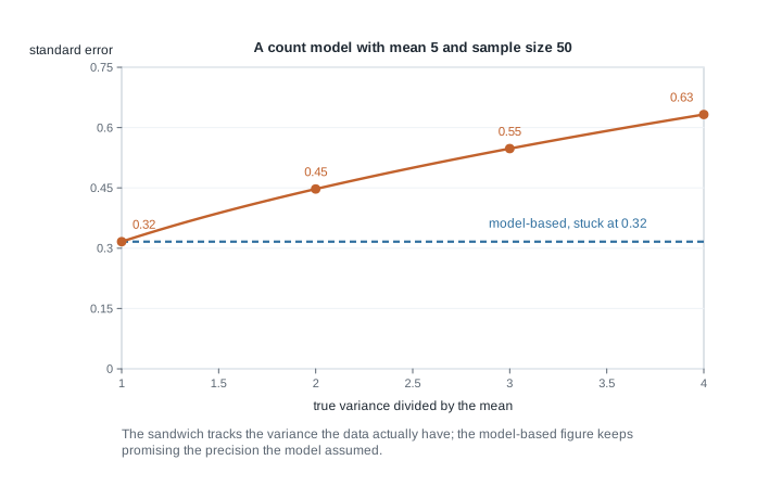
The figure is the simplest exact instance. A count response is modelled as Poisson with mean \(\mu = 5\) and \(n = 50\), so the score equation is the one defining the sample mean, but the true variance is \(\tau \mu\) for a dispersion \(\tau \ge 1\). The model-based standard error is \(\sqrt{\mu / n} = \sqrt{5/50} = 0.32\) whatever \(\tau\) is, while the sandwich returns \(\sqrt{\tau \mu / n} = 0.32 \sqrt{\tau}\): \(0.45\) at \(\tau = 2\) and \(0.63\) at \(\tau = 4\), so the model-based width is out by a factor of two at \(\tau = 4\).

Note

Here the sandwich repaired the standard error and the estimand survived, because the Poisson score equation targets the mean whatever the variance is. That is the favourable case, not the general one. In a logistic regression with an omitted covariate, the fitted coefficient targets a marginal log-odds ratio that generally differs from the conditional one the model was written to describe, and the sandwich gives an impeccable standard error for a quantity nobody set out to estimate.

Worked example — influence functions for the mean and the median

Let \(X_1, \dots, X_n\) be independent with distribution \(F\) whose density \(f\) is continuous and strictly positive near its median \(m\), so that \(m\) is the unique solution of \(F(m) = 1/2\). Compare the influence functions of the mean and median functionals at this \(F\), then check the comparison against the ten laboratory readings from the top of the page.

Step 1: the mean, exactly. The mean functional is linear in \(F\), so \(\mu(F_\varepsilon) = (1 - \varepsilon) \mu + \varepsilon x\) and the difference quotient is \(x - \mu\) for every \(\varepsilon\), not only in the limit. Hence \(\mathrm{IF}(x; \mu, F) = x - \mu\), which grows without bound in \(\lvert x \rvert\), so \(\gamma^{*} = \infty\).

Step 2: the median, implicitly. The contaminated median satisfies \(F_\varepsilon(m_\varepsilon) = 1/2\), that is \((1 - \varepsilon) F(m_\varepsilon) + \varepsilon \, \mathbf{1}\{x \le m_\varepsilon\} = 1/2\). Fix \(x \ne m\), so the indicator is locally constant in \(\varepsilon\), and differentiate at \(\varepsilon = 0\) using \(F(m) = 1/2\) and continuity of \(f\) at \(m\):

\[-F(m) + f(m) \, m'(0) + \mathbf{1}\{x \le m\} = 0 \quad \Longrightarrow \quad m'(0) = \frac{1/2 - \mathbf{1}\{x \le m\}}{f(m)} .\]

For \(x > m\) the indicator is zero and the derivative is \(1 / (2 f(m))\); for \(x < m\) it is \(-1 / (2 f(m))\). Hence \(\mathrm{IF}(x; m, F) = \mathrm{sign}(x - m) / (2 f(m))\) and \(\gamma^{*} = 1 / (2 f(m))\), finite. Notice where the conditions do their work: if \(f(m) = 0\) the derivative blows up, and if \(F\) has an atom at \(m\) the implicit relation is not differentiable at all. Bounded influence for the median is a property of \(F\) as much as of the median.

Step 3: what the two say about variance. Squaring and integrating gives \(\int (y - \mu)^2 dF = \sigma^2\) for the mean, reproducing the central limit theorem, and \(1 / (4 f(m)^2)\) for the median. At \(N(\theta, \sigma^2)\), \(f(m) = 1 / (\sigma \sqrt{2\pi})\), so the median’s asymptotic variance is \(\pi \sigma^2 / 2 \approx 1.571 \sigma^2\) and its sensitivity is \(\sigma \sqrt{2\pi} / 2 \approx 1.253 \sigma\); the asymptotic relative efficiency of the median to the mean at the normal is \(2/\pi \approx 0.637\).

Influence functions of the mean, the median, and the Huber estimator at the standard normal model.

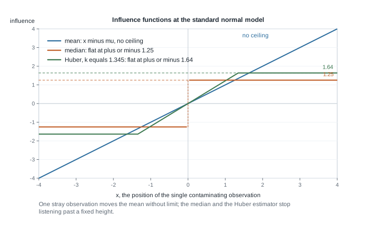
Step 4: the same contrast on ten numbers. Replacing one observation of \(n\) by a value \(x\) changes the sample mean by exactly \((x - x_{\text{old}}) / n\), which for the transposed digit is \((61 - 16)/10 = 4.5\): the mean moves from \(9.6\) to \(14.1\), the unbounded linear response the influence function predicts. The sample median is \(8.5\) before and after, because the fifth and sixth ordered values, \(8\) and \(9\), were not touched.

What this licenses: a quantitative statement of how far one contaminating value can move each estimator, and a variance comparison at any \(F\) where \(f(m)\) is known. What it does not license: any claim that the median is “better”. At the clean normal it is nearly \(57\) per cent more expensive in sample size, and the sample median at finite \(n\) is a non-smooth function of the data, depending on only one or two order statistics rather than on all of them the way the influence-function expansion suggests.

The same reasoning, transferred

Run the identical derivation at a skewed model. Let \(X_1, \dots, X_n\) be exponential with rate \(\lambda\), so \(f(y) = \lambda e^{-\lambda y}\) for \(y > 0\). The median solves \(1 - e^{-\lambda m} = 1/2\), giving \(m = \log 2 / \lambda\), and the density there is \(f(m) = \lambda e^{-\lambda m} = \lambda / 2\). Substituting into the formula from Step 2 gives \(\mathrm{IF}(x; m, F) = \mathrm{sign}(x - m) / \lambda\), so \(\gamma^{*} = 1/\lambda\) and the median’s asymptotic variance is \(1 / (4 f(m)^2) = 1/\lambda^2\). For the mean, \(\mathrm{IF}(x) = x - 1/\lambda\) with infinite sensitivity and asymptotic variance \(\mathrm{Var}(X) = 1/\lambda^2\).

What stayed the same is the argument: differentiate the defining relation, evaluate the density at the target, read off the two summaries. What changed is decisive. The two functionals no longer agree — the mean is \(1/\lambda\), the median \(0.693/\lambda\), a factor of \(1/\log 2 \approx 1.44\) apart — so switching to the median does not estimate the same quantity more safely, it estimates a different quantity. And the median buys no variance reduction here, both asymptotic variances being \(1/\lambda^2\); the entire gain is bounded influence. At an asymmetric model the choice of functional is a modelling decision, not a technical safeguard.

Second worked example — a Huber estimate on a contaminated sample

Take the corrupted readings \(x = (4, 7, 7, 7, 8, 9, 10, 14, 14, 61)\) and fit the Huber location estimator with the scale held fixed, which is what makes the arithmetic checkable by hand. The scale comes from a preliminary high-breakdown estimate: the median absolute deviation of these readings about their median is \(1.5\), the same before and after the corruption, so the consistency-corrected scale is \(1.5 / 0.6745 = 2.22\) and the standard tuning gives \(k = 1.345 \times 2.22 = 2.99\). Round it to \(k = 3\) in the measurement’s own units, treat it as fixed, and solve

\[\sum_{i=1}^{10} \psi_3(x_i - \theta) = 0 .\]

Step 1: an iteration you can run by hand. Adding \(\theta\) to each clipped residual puts the estimating equation in fixed-point form: \(\theta^{(m+1)} = \theta^{(m)} + \frac{1}{n} \sum_i \psi_3(x_i - \theta^{(m)})\), which is the mean of the readings winsorized — pulled in — to the window \([\theta^{(m)} - 3, \theta^{(m)} + 3]\). From \(\theta^{(0)} = 8.5\), the median, the iterates are \(8.8\), \(8.92\), \(8.968\), \(8.9872\), \(8.99488\).

Step 2: solve it exactly instead. From the first step onward the classification never changes: one reading (\(4\)) sits below the window, six (\(7, 7, 7, 8, 9, 10\)) inside, three (\(14, 14, 61\)) above. There the update is the affine map \(\theta \mapsto [(\theta - 3) + 48 + 3(\theta + 3)]/10 = 0.4 \theta + 5.4\), whose unique fixed point is \(\hat\theta = 9.0\). Confirm it directly: at \(\theta = 9\) the values of \(\psi_3(x_i - 9)\) are \(-3, -2, -2, -2, -1, 0, 1, 3, 3, 3\), summing to zero. The contraction factor \(0.4\) is exactly \(1 - \hat{A}\) with \(\hat{A} = 6/10\), which is why the plain iteration converges steadily but not quickly.

Step 3: compare the four estimates. On the corrupted data the sample mean is \(14.1\), the median \(8.5\), the ten per cent trimmed mean \(9.5\), the Huber estimate \(9.0\). Repeat on the uncorrupted readings, whose last value is \(16\): mean \(9.6\), median \(8.5\), trimmed mean \(9.5\), and Huber estimate again \(9.0\) — because \(16\) and \(61\) both lie beyond \(\hat\theta + k = 12\) and clip to the same \(+3\). The estimating function cannot tell them apart, which is the whole design.

The same ten readings before and after one digit transposition, with the mean, median, and Huber estimate marked on each.

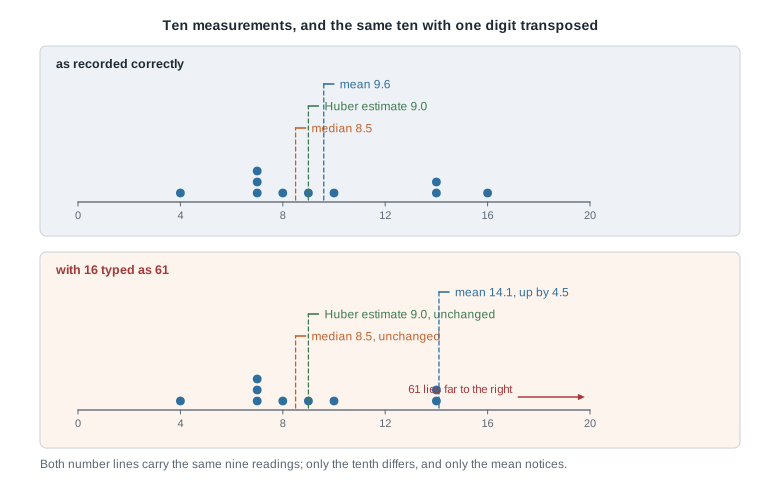
Step 4: a standard error that survives too. With \(\hat\theta = 9\) and \(k = 3\) the squared clipped residuals are \(9, 4, 4, 4, 1, 0, 1, 9, 9, 9\), summing to \(50\), so \(\hat{B} = 5.0\); six of the ten readings lie strictly within \(3\) of \(\hat\theta\), so \(\hat{A} = 0.6\). Then \(\hat{A}^{-1} \hat{B} \hat{A}^{-1} = 5.0 / 0.36 = 13.89\) and the standard error of \(\hat\theta\) is \(\sqrt{13.89 / 10} = 1.18\), giving the approximate interval \(9.0 \pm 1.96 \times 1.18 = (6.69, 11.31)\) against the corrupted-data \(t\) interval \((2.10, 26.10)\). On the uncorrupted readings every one of those numbers is identical, since \(16\) and \(61\) clip to the same value.

psi <- function(u, k) pmax(-k, pmin(u, k))

huber_location <- function(x, k, start = median(x), tol = 1e-12) {
  theta <- start
  repeat {
    step <- mean(psi(x - theta, k))
    theta <- theta + step
    if (abs(step) < tol) break
  }
  theta
}

sandwich_se <- function(x, theta, k) {
  meat  <- mean(psi(x - theta, k)^2)
  bread <- mean(abs(x - theta) < k)
  sqrt(meat / bread^2 / length(x))
}

x <- c(4, 7, 7, 7, 8, 9, 10, 14, 14, 61)
huber_location(x, k = 3)            # 9
sandwich_se(x, theta = 9, k = 3)    # 1.1785

What this licenses: an estimate and an interval for the Huber functional of \(F\) that a single gross error cannot move, and a diagnostic — the gap between \(9.0\) and \(14.1\) — that flags the corruption without anyone deleting a number. What it does not license: the \(1.96\) is an asymptotic quantile used at \(n = 10\) and \(\hat{B}\) is a noisy average of ten terms, so the interval is optimistic; the Huber functional equals the mean of \(F\) only when \(F\) is symmetric about it, so under one-sided contamination the estimate is a boundedly biased version of the clean mean; and \(\hat{A}\) needs a convention when a residual falls exactly at \(\pm k\), though here none does.

The misreading to avoid

The sentence to dismantle gets written in methods sections every week: “we used robust standard errors, so misspecification is not a concern.” Put more carefully — “the sandwich estimator is consistent under misspecification” — it is true and still leads to the same mistake, because the phrase quietly omits consistent for what.

The correct version. The M-estimator converges to \(\theta_0\), the root of \(\int \psi(y, \theta) \, dF(y) = 0\) under the true \(F\), and the sandwich gives a valid standard error for that \(\theta_0\). If the model is right, \(\theta_0\) is the parameter you wanted. If the model is wrong, \(\theta_0\) is whatever the estimating equation defines at the true \(F\) — for a likelihood score, the value minimizing Kullback-Leibler divergence from \(F\) to the model family — and a valid standard error for the wrong quantity is not a repair. The sandwich fixes the variance, not the estimand. The overdispersed-Poisson case is benign only because the estimand happens to survive; the omitted-covariate logistic case is not, and the two outputs look identical.

A second misreading rides along: “robust methods are strictly safer, so use them by default.” Robustness is a purchase, not a discount, and the table above prices it — about \(57\) per cent more sample size for the median at an exactly normal model, about five per cent for a well-tuned Huber estimator. A third variant substitutes deletion for estimation: find the outlier, drop it, run the \(t\) procedure, and report a standard error computed as though the deletion had not been a data-dependent choice. That is the selective-inference error of Week 9 in new clothing.

Finally, “distribution-free” and “robust” are not synonyms, and neither means assumption-free. The M-estimator here still assumes independence, still needs a scale, still needs a unique root, and still reports an asymptotic approximation. Robustness buys insensitivity to one stated departure — contamination of the central model — and nothing else comes free with it.

Practice on your own

1. Derive the influence function of the variance functional \(\sigma^2(F) = \int (y - \mu(F))^2 dF(y)\) at a distribution with finite fourth moment, by writing \(\sigma^2(F_\varepsilon)\) out and differentiating at \(\varepsilon = 0\). Check that it integrates to zero under \(F\), and say what its growth in \(x\) implies for the sample standard deviation, which moves from \(3.864\) to \(16.776\) between the two samples above.
2. Compute the finite-sample replacement breakdown point of the midrange \((x_{(n)} + x_{(1)})/2\) and of the twenty per cent trimmed mean at \(n = 10\). Then construct a distribution and a contamination fraction of \(0.1\) at which the trimmed mean, despite its healthy breakdown point, is worse than that number alone would suggest.
3. Take \(X\) normal with mean \(\theta\) and known variance \(\sigma^2\), and \(\psi(x, \theta) = (x - \theta)/\sigma^2\), the score. Show \(A = B = 1/\sigma^2\), so the sandwich collapses to \(\sigma^2\). Now let the data have variance \(\tau^2 \ne \sigma^2\) with \(\psi\) unchanged: recompute \(A\) and \(B\), and confirm the sandwich returns \(\tau^2\) while the model-based variance still reports \(\sigma^2\).
4. Re-solve the estimating equation of the second worked example by hand with \(k = 1.5\) instead of \(k = 3\). Can you predict from the shape of \(\psi_k\), before computing, which way the estimate moves?
5. Run the contamination study below and compare its columns against the asymptotic variances tabulated earlier. Then repeat with the contaminating component shifted rather than widened, using rnorm(n, mean = 8) for the contaminated draws, and explain why the ordering changes.

set.seed(2027)
draw <- function(n, eps, spread) {
  bad <- rbinom(n, 1, eps)
  rnorm(n, mean = 0, sd = ifelse(bad == 1, spread, 1))
}
one_run <- function(n, eps, spread) {
  z <- draw(n, eps, spread)
  c(mean = mean(z), trimmed = mean(z, trim = 0.1),
    median = median(z), huber = huber_location(z, k = 1.345))
}
study <- replicate(4000, one_run(50, 0.10, 3))
50 * apply(study, 1, var)   # compare with the asymptotic variances in the table

Where to read more

• The asymptotic machinery behind M-estimation — estimating equations, the delta method, and the sandwich — is developed at graduate level in MIT OpenCourseWare 18.655 Mathematical Statistics, the natural place to see the regularity conditions written out in full.
• For the fundamentals this week perturbs — the sample mean, its standard error, and the \(t\) interval whose fragility opened the unit — see Penn State STAT 415.
• The optional Hogg, McKean, and Craig alignment for this week is Chapter 10.6 through 10.9. The book is optional and never required for this course; availability and licence terms for every source listed here remain unconfirmed.
• Computing needs nothing beyond The R Project for Statistical Computing and Quarto; every block on this page runs in base R and stats.
• Course pages: the notes overview, the syllabus, the schedule, and the resources page.

Where this goes next

The last piece of this week is a bridge you have half-built already. Choosing a procedure by how badly it can behave across a whole neighbourhood, rather than by how well it behaves at one distribution, is a minimax argument: the neighbourhood plays the part the parameter space plays in Week 1’s risk functions, and Huber’s original result was that his estimator minimizes the maximum asymptotic variance over a gross-error neighbourhood of the normal. Week 14 takes that home — Bayes rules as minimizers of posterior expected loss, admissibility, minimaxity through least-favourable priors, and the Stein phenomenon. Influence functions will not appear there, but the habit of judging an estimator by a whole risk curve rather than one number will.

Carry two threads forward. As soon as a procedure is defined by an estimating equation rather than by a model, you owe the reader a statement of which functional it targets; and every robustness gain is paid for in efficiency at the clean model, at a price computable in advance. Both return in Week 15, where one target is worked five ways with the rank-based route among them. If the influence-function derivations felt like sleight of hand, revisit the plug-in of Week 11, and use the notes overview to see where this unit sits after Week 12.