Week 11 — Bootstrap, jackknife, and resampling calibration
Where this week starts
Week 10 bought exactness with design: if the assignment of units to treatments really was random, the randomization distribution of a statistic is known by enumeration and a permutation test has exact size with no distributional assumption. That guarantee is strong and narrow, since it needs a mechanism you controlled and tests a sharp null rather than a parameter. Weeks 5 and 6 bought generality with asymptotics instead, charging for it in conditions and in a calibration only as good as your sample size makes it.
Between those lies the case that fills a working week. Your estimand is a feature of a distribution rather than a parameter of a named family: a ratio of means, a median, a correlation. There is no monotone likelihood ratio to exploit, no pivot to invert, no randomization you performed, and usually no tractable sampling distribution. What you do have is the sample, and this week’s idea is to let it stand in for the population: write the estimand as a functional of the unknown distribution, replace that distribution by the empirical distribution of your data, and the experiment you could never repeat becomes one you can repeat at will.
What should feel different by the end is the question you ask when a resampling result looks wrong: not “does the bootstrap work here” but “which of the two approximations is failing”. There are exactly two, and only one is cured by a faster computer.
Why this matters beyond the theorem
Six plots of a field trial are measured for area and yield, and a percentile bootstrap interval for yield per unit area runs from 2.35 to 2.82 around an estimate of 2.50. Somebody writes: there is a 95 percent probability that the true ratio lies between 2.35 and 2.82. Two things have gone wrong. The first is interpretive: that interval came from a conditional distribution of recomputed estimates given the data in hand, not from a posterior, which would need a prior this analysis never supplied. The second is calibration: for a skewed functional at a small sample size the percentile construction does not cover at its nominal rate, and the simulation below puts its coverage near 0.87 at a sample size of ten.
Failure can be worse than a shortfall. For one ordinary estimand — the largest value a population can take, estimated by the largest observed — the percentile interval has coverage exactly zero at every sample size, for a reason you can compute in one line.
What you will be able to do
- Derive the basic, percentile, and studentized intervals from the pivotal quantity each one inverts, and state the assumption under which each is correct.
- Compute an exact bootstrap distribution for a small sample by enumeration, and read all three intervals off it.
- Separate simulation error, which more resamples remove, from statistical error, which they do not, and attach a number to each.
- Estimate bias and variance by the jackknife, and verify that the deletion formulas reproduce the second-order bias expansion and the delta-method variance.
- Diagnose an estimand for which the bootstrap is inconsistent and name the property that breaks it.
- Design a coverage study, report its Monte Carlo standard error, and decide whether a shortfall is real.
Terms and notation worth fixing
| Symbol | What it means on this page |
|---|---|
| \(F\), \(\hat F_n\) | The population distribution, and the empirical distribution placing mass \(1/n\) on each observed value |
| \(T\), \(\theta = T(F)\) | A functional of a distribution, and the estimand it defines |
| \(\hat\theta = T(\hat F_n)\) | The plug-in estimator: the identical functional evaluated at \(\hat F_n\) |
| \(\hat\theta^*\) | The same estimator on one resample of size \(n\) drawn with replacement |
| \(P^*\) | Probability in the resampling world, conditional on the observed data |
| \(q^*_p\) | The \(p\) quantile of the bootstrap distribution: the smallest \(t\) with \(P^*(\hat\theta^* \le t) \ge p\) |
| \(B\), \(R\) | Resamples inside one bootstrap, and replicate data sets in a calibration study |
| \(\hat\theta_{(i)}\), \(\hat\theta_{(\cdot)}\) | The estimator with observation \(i\) deleted, and the average of those \(n\) values |
The plug-in principle and the bootstrap analogy
Start with the substitution itself: every method this week is a special case of it, and every failure this week is a failure of it.
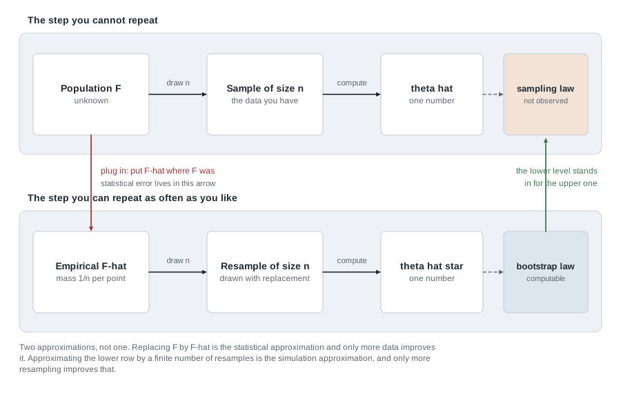
The upper row is the experiment that produced your data, which you cannot rerun. The lower row is the same experiment with \(\hat F_n\) in place of \(F\), and it can be rerun freely, since sampling from \(\hat F_n\) is drawing from a list of \(n\) numbers with replacement. The red arrow between the rows carries the entire statistical content of the method.
Estimating a functional by plugging in the sample
The mean is \(T(F) = \int x \, dF(x)\), the median is \(T(F) = F^{-1}(1/2)\), and the ratio this page works with is \(T(F) = \mu_Y(F)/\mu_X(F)\) for a bivariate \(F\). In each case the plug-in estimator is the same expression at \(\hat F_n\): one rule generates all of them, and applies to resampled data just as easily.
Why should this converge? Two conditions do the work. First, \(\hat F_n\) converges to \(F\) uniformly: Glivenko-Cantelli gives \(\sup_x |\hat F_n(x) - F(x)| \to 0\) almost surely for independent and identically distributed observations, with no assumption on \(F\) beyond that. Second, \(T\) must be continuous at \(F\) in a topology that statement controls. The second is a real restriction: the mean is not continuous in the supremum metric without a moment condition, and the upper endpoint of the support is not continuous in any useful sense at all.
The bootstrap goes further and plugs in for the whole sampling distribution. You want the law of \(\hat\theta - \theta\) under \(F\); you compute the law of \(\hat\theta^* - \hat\theta\) under \(\hat F_n\), which is fully known once the data are in hand — a distribution over \(n^n\) equally likely resamples, written down exactly rather than simulated when \(n\) is small.
Two approximations, and only one of them shrinks with computing
Every bootstrap number carries two distinct errors, and confusing them is the technical mistake of the week. The statistical error is the difference between the law of \(\hat\theta^* - \hat\theta\) under \(\hat F_n\) and the law of \(\hat\theta - \theta\) under \(F\). It exists because \(\hat F_n\) is not \(F\); it shrinks when \(n\) grows and not at all when you draw more resamples, which tell you only about \(\hat F_n\). The simulation error is the difference between the exact bootstrap distribution and the empirical distribution of the \(B\) resamples you drew. It shrinks at rate \(B^{-1/2}\) and is a budget decision, not a statistical quantity.
The same split governs Monte Carlo testing. Let \(T_{\text{obs}}\) be observed and \(T_1, \dots, T_B\) generated under the null so that the \(B + 1\) values are exchangeable when the null holds. Then
\[ \hat p = \frac{1 + \#\{b : T_b \ge T_{\text{obs}}\}}{B + 1} \]
satisfies \(P(\hat p \le \alpha) \le \alpha\) under the null, with equality when \(\alpha(B + 1)\) is an integer and ties among the \(B + 1\) values have probability zero. The two additions of one are what make this exact; dividing by \(B\), or dropping the leading one, gives a test whose size can exceed \(\alpha\). Here simulation error costs power, never validity, a different bargain from the intervals below.
Three intervals from one bootstrap distribution
One bootstrap distribution supports several intervals, and they are genuinely different procedures: each inverts a different quantity and each is exactly right under a different assumption.
Basic and percentile intervals as two inversions
The basic interval treats \(\hat\theta - \theta\) as an approximate pivot. If you knew \(a\) and \(b\) with \(P(a \le \hat\theta - \theta \le b) = 1 - \alpha\), rearranging inside the probability gives \(\hat\theta - b \le \theta \le \hat\theta - a\). Estimate them in the resampling world, where the analogue is \(\hat\theta^* - \hat\theta\): take \(a = q^*_{\alpha/2} - \hat\theta\) and \(b = q^*_{1-\alpha/2} - \hat\theta\), giving
\[ \left( 2\hat\theta - q^*_{1-\alpha/2}, \; 2\hat\theta - q^*_{\alpha/2} \right). \]
Read the subscripts twice: the upper endpoint uses the lower bootstrap quantile. That reversal is the rearrangement above, and it is why the basic interval reaches in the direction opposite to the bootstrap distribution’s own skew.
The percentile interval is the pair of bootstrap quantiles themselves, \((q^*_{\alpha/2}, q^*_{1-\alpha/2})\), with no reflection. This looks like a shortcut and is a different claim, exactly correct under this condition: there exists a strictly increasing \(g\) with \(g(\hat\theta) - g(\theta)\) distributed symmetrically about zero and free of \(\theta\), and the bootstrap reproduces that distribution for \(g(\hat\theta^*) - g(\hat\theta)\). You never have to find \(g\), which is the appeal; when no such \(g\) exists the interval has no justification, and nothing in the picture reveals that.
One consequence is worth memorizing. Quantiles commute with increasing transformations, so the percentile interval for \(m(\theta)\) is the image under \(m\) of the percentile interval for \(\theta\); the basic interval has no such property, since reflecting through \(\hat\theta\) does not commute with a nonlinear \(m\).
The studentized interval and second-order accuracy
The studentized interval, or bootstrap-\(t\), pivots on a scaled quantity. With \(\widehat{\mathrm{se}}\) a standard error computed from the data and \(\widehat{\mathrm{se}}^*\) the same formula on each resample, form \(t^* = (\hat\theta^* - \hat\theta)/\widehat{\mathrm{se}}^*\), take its bootstrap quantiles, and invert as before:
\[ \left( \hat\theta - \widehat{\mathrm{se}} \cdot t^*_{1-\alpha/2}, \; \hat\theta - \widehat{\mathrm{se}} \cdot t^*_{\alpha/2} \right). \]
The tails are again reversed. What this buys is accuracy: under the smooth function model — \(\theta = g(\mu)\) for a sufficiently smooth \(g\) and a population mean vector \(\mu\), with enough finite moments and a non-lattice condition on the underlying distribution — an Edgeworth expansion gives the studentized interval a one-sided coverage error of order \(n^{-1}\), against \(n^{-1/2}\) for the percentile and basic intervals. It corrects for skewness automatically.
What it costs is a standard error for every resample: free for a mean or a ratio, severe for a median, where no simple plug-in exists and each resample needs its own inner bootstrap. It also costs stability, because dividing by a small estimated standard error produces enormous studentized values, which at small \(n\) fattens the tails of \(t^*\) and lengthens the interval.
The jackknife, deletion, and smooth functionals
The jackknife predates the bootstrap and asks a narrower question with \(n\) recomputations rather than thousands. It estimates bias and variance, and works when the functional is smooth enough for a first-order expansion to be faithful.
Bias from n deletions
Suppose the bias expands in powers of \(1/n\), which holds for smooth functions of sample moments and fails for others:
\[ E_\theta(\hat\theta_n) = \theta + \frac{a(\theta)}{n} + \frac{b(\theta)}{n^2} + O(n^{-3}). \]
Each \(\hat\theta_{(i)}\) is the same rule on \(n - 1\) observations, so \(E_\theta(\hat\theta_{(\cdot)}) = \theta + a/(n-1) + b/(n-1)^2 + O(n^{-3})\), and therefore
\[ E_\theta\left\{ (n-1)\left( \hat\theta_{(\cdot)} - \hat\theta_n \right) \right\} = (n-1)\left( \frac{a}{n-1} - \frac{a}{n} \right) + O(n^{-2}) = \frac{a}{n} + O(n^{-2}), \]
which is exactly the leading bias term, and is where the factor \(n - 1\) comes from. So \(\widehat{\mathrm{bias}} = (n-1)(\hat\theta_{(\cdot)} - \hat\theta_n)\) and the corrected estimator \(\tilde\theta = n\hat\theta_n - (n-1)\hat\theta_{(\cdot)}\) has bias of order \(n^{-2}\). Correction is not free: subtracting an estimated quantity adds variance, and the corrected estimator can have the larger mean squared error.
Variance, and where deletion fails
The jackknife variance estimate is
\[ v_{\text{jack}} = \frac{n-1}{n} \sum_{i=1}^{n} \left( \hat\theta_{(i)} - \hat\theta_{(\cdot)} \right)^2 . \]
The factor \((n-1)/n\) is there because deletion produces differences too small by a factor of about \(n - 1\); the identity \(\bar{x}_{(i)} - \bar{x} = -(x_i - \bar{x})/(n-1)\), worth verifying once by hand, shows why. For a smooth functional the estimate agrees with the delta method to first order, as the second worked example checks numerically.
Deletion fails when the functional is not smooth, and the standard counterexample is the median. Deleting one observation moves the median to a neighbouring order statistic or not at all, so the \(n\) deleted values take two or three distinct values whose spread misdescribes the sampling variability: the jackknife variance estimate for the median is inconsistent. The repair, stated and not developed here, is to delete blocks of \(d\) observations with \(d\) growing with \(n\). Deletion assumes local linearity of the functional in the empirical distribution.
Worked example — a bootstrap interval for a ratio of means
The model and the question. Six plots in a field trial are recorded with area \(x_i\) in hectares and yield \(y_i\) in tonnes, treated as independent draws from an unknown bivariate \(F\). The estimand is \(\theta = \mu_Y / \mu_X\), the yield per hectare a very large trial would report. The areas are \(0.5, 0.8, 1.0, 1.2, 1.5, 2.0\) and the yields \(1.9, 2.0, 2.4, 3.0, 3.4, 4.8\). Nothing is assumed about the shape of \(F\), so no exact procedure from Weeks 2 through 4 applies, and at six observations no asymptotic argument deserves much trust either.
Step 1: the plug-in estimate. Areas sum to \(7.0\) and yields to \(17.5\), so \(\hat\theta = 17.5/7.0 = 2.50\). A ratio of means is not a mean of ratios: the six per-plot ratios \(3.800, 2.500, 2.400, 2.500, 2.267, 2.400\) average \(2.644\) instead, and the first plot — small and unusually productive — is going to matter.
Step 2: an analytic standard error. Write \(r_i = y_i - \hat\theta x_i\); because \(\hat\theta = \bar{y}/\bar{x}\) these sum to zero exactly. A one-term expansion gives \(\hat\theta - \theta \approx (\bar{y} - \theta\bar{x})/\mu_X\), so
\[ \widehat{\mathrm{se}}(\hat\theta) = \frac{1}{\bar{x}} \sqrt{\frac{\sum_{i=1}^{n} r_i^2}{n(n-1)}} . \]
The residuals are \(0.65, 0.00, -0.10, 0.00, -0.35, -0.20\), summing to zero, and their squares sum to \(0.595\). With \(n = 6\) and \(\bar{x} = 7/6\) this is \(\sqrt{0.595/30}\,/\,(7/6) = 0.1408/1.1667 = 0.1207\). A large-sample interval would be \(2.50 \pm 1.96 \times 0.1207\), from \(2.263\) to \(2.737\).
Step 3: the bootstrap distribution, computed rather than simulated. A resample draws six of the six pairs with replacement, giving \(6^6 = 46{,}656\) equally likely resamples — few enough to enumerate, so this example carries no simulation error at all. Enumeration gives \(376\) distinct values of \(\hat\theta^*\), from \(2.267\) to \(3.800\), with mean \(2.516\), standard deviation \(0.127\), and skewness \(1.43\).
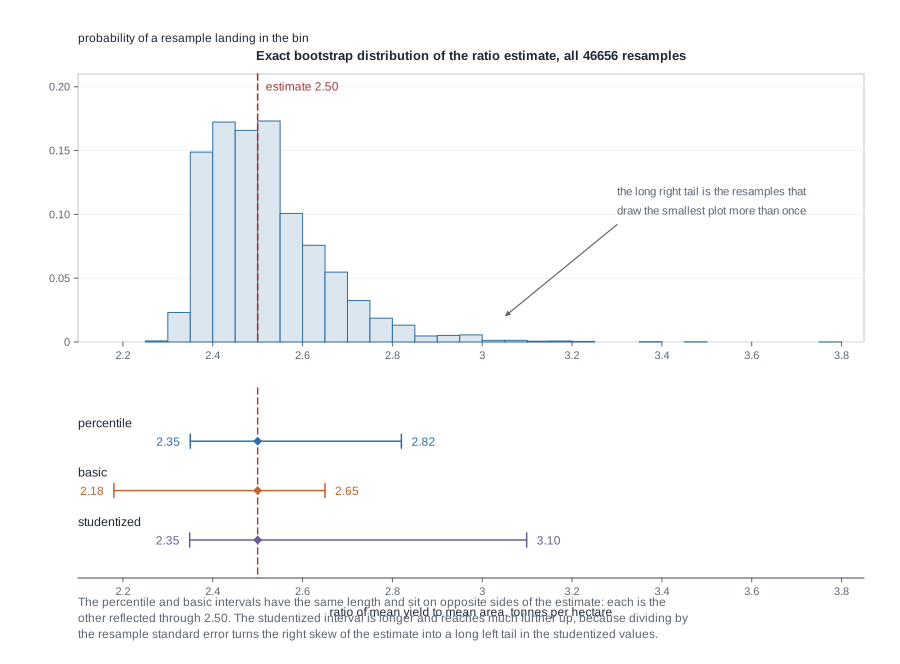
The skew has a concrete cause: resamples drawing the first plot zero, one, two, or three times average \(2.402\), \(2.504\), \(2.632\), and \(2.798\), and a fraction \((5/6)^6 = 0.335\) omit it entirely. One influential pair generates the tail.
Step 4: the percentile and basic intervals. With the quantile convention in the notation table, \(q^*_{0.025} = 2.35\) and \(q^*_{0.975} = 2.82\), so the percentile interval runs from \(2.35\) to \(2.82\). The bootstrap distribution is discrete, so no interval carries exactly 95 percent of its mass; this one carries \(0.9531\). Reflecting through \(\hat\theta\) gives \(2 \times 2.50 - 2.82 = 2.18\) and \(2 \times 2.50 - 2.35 = 2.65\). Both intervals have length \(0.47\) and sit on opposite sides of the estimate; they would coincide if the bootstrap distribution were symmetric about \(\hat\theta\).
Step 5: the studentized interval. Recomputing the Step 2 formula inside each resample and forming \(t^* = (\hat\theta^* - \hat\theta)/\widehat{\mathrm{se}}^*\) gives \(t^*_{0.025} = -4.96\) and \(t^*_{0.975} = 1.25\). Inverting, the endpoints are \(2.50 - 0.1207 \times 1.25 = 2.35\) and \(2.50 + 0.1207 \times 4.96 = 3.10\). One honest detail: \(130\) of the \(46{,}656\) resamples draw only pairs sharing a common yield-to-area ratio, making \(\widehat{\mathrm{se}}^*\) exactly zero and \(t^*\) undefined; excluding them, rather than pushing them to either extreme, moves each endpoint by less than \(0.01\).
What this licenses, and what it does not. Three procedures, one data set, three intervals. Each is a repeated-sampling statement: if the trial were repeated many times and the interval recomputed, a certain fraction would contain \(\theta\). None is a probability statement about \(\theta\) given this trial, and “a certain fraction” is doing real work, because nothing so far establishes that the fraction is 0.95.
The same reasoning, transferred
Run the identical construction on the log scale, where the estimand is \(\log\theta\) and the estimate is \(\log\hat\theta = 0.9163\). What stays the same: the \(46{,}656\) resamples with their probabilities, and the two inversion formulas. What changes: only the functional.
Because the logarithm is increasing, the bootstrap quantiles of \(\log\hat\theta^*\) are the logarithms of those of \(\hat\theta^*\). The percentile interval on the log scale therefore runs from \(\log 2.35\) to \(\log 2.82\), and exponentiating returns exactly \(2.35\) to \(2.82\): the same interval as before. The basic interval is not equivariant. On the log scale it is \(2 \times 0.9163 - 1.0367 = 0.7959\) to \(2 \times 0.9163 - 0.8544 = 0.9782\), and exponentiating gives \(2.216\) to \(2.660\), not the \(2.18\) to \(2.65\) obtained on the original scale. Two analysts using one method on one data set disagree because one took a logarithm first: reflection through \(\hat\theta\) is linear and a logarithm is not, so they do not commute — the same reason the Wald statistic of Week 5 depends on parameterization and the likelihood-ratio statistic does not.
Second worked example — the jackknife bias of an estimated rate
The model and the question. A reliability test runs five components to failure, with lifetimes \(2, 3, 4, 5, 6\) in thousands of hours. The estimand is the failure rate \(\theta = 1/\mu\), estimated by \(\hat\theta = 1/\bar{x}\). Since \(1/x\) is convex, Jensen’s inequality gives \(E(1/\bar{X}) > 1/\mu\), so the estimator is biased upward. By how much, without a parametric model?
Step 1: the ingredients. The lifetimes sum to \(20\), so \(\bar{x} = 4\) and \(\hat\theta = 0.25\). The deviations are \(-2, -1, 0, 1, 2\), so \(\sum (x_i - \bar{x})^2 = 10\) and \(s^2 = 10/4 = 2.5\).
Step 2: the five deleted estimates. Deleting one observation at a time leaves means \(18/4 = 4.5\), \(17/4 = 4.25\), \(16/4 = 4\), \(15/4 = 3.75\), \(14/4 = 3.5\), so the deleted estimates are \(0.222222\), \(0.235294\), \(0.250000\), \(0.266667\), \(0.285714\), summing to \(1.259897\) with average \(\hat\theta_{(\cdot)} = 0.251979\).
Step 3: the jackknife bias estimate. \(\widehat{\mathrm{bias}} = 4 \times (0.251979 - 0.25) = 0.007918\), so the corrected estimate is \(0.25 - 0.007918 = 0.242082\). No model entered, only the five numbers.
Step 4: the theoretical bias. Expanding \(g(t) = 1/t\) about \(\mu\) to second order, \(E\{g(\bar{X})\} \approx 1/\mu + \sigma^2/(n\mu^3)\), so the leading bias is \(\sigma^2/(n\mu^3)\), with plug-in version \(s^2/(n\bar{x}^3) = 2.5/(5 \times 64) = 0.0078125\). Against the jackknife’s \(0.0079179\) that is a difference of about one and a half percent, which is the third-order term the expansion dropped. The agreement is not luck: substituting \(\bar{x}_{(i)} - \bar{x} = -(x_i - \bar{x})/(n-1)\) into the same expansion gives \((n-1)(\hat\theta_{(\cdot)} - \hat\theta) \approx s^2/(n\bar{x}^3)\) algebraically.
Step 5: the jackknife variance. The deleted estimates deviate from their average by \(-0.029757, -0.016685, -0.001979, 0.014687, 0.033735\), whose squares sum to \(0.00252155\). Multiplying by \((n-1)/n = 0.8\) gives \(v_{\text{jack}} = 0.0020172\) and a standard error of \(0.04491\). The delta method predicts \(\sigma^2/(n\mu^4)\), estimated by \(2.5/(5 \times 256) = 0.0019531\) and a standard error of \(0.04419\), as the general argument said it must.
What this licenses, and what it does not. Had you assumed exponential lifetimes, \(n\bar{X}\) would be gamma and \(E(1/\bar{X}) = n\lambda/(n-1)\) exactly, making the bias \(\lambda/(n-1)\), which at \(\hat\lambda = 0.25\) and \(n = 5\) is \(0.0625\) — eight times the jackknife’s number. That is the right bias for the wrong model: these lifetimes have standard deviation \(1.58\) while an exponential population with mean \(4\) has standard deviation \(4\). Estimating bias at the distribution the data actually came from is the jackknife’s whole claim.
Calibration: what these intervals actually cover
Construction is not calibration. To learn what the three constructions cover, generate data from a known population, build all three, and count. The study below takes the simplest skewed case: independent draws from an exponential population with mean one, estimand the population mean, four sample sizes, \(B = 999\) resamples inside each of \(R = 5000\) replicates, nominal level 0.95.
one_replicate <- function(n, B = 999) {
  x  <- rexp(n)
  bs <- replicate(B, { r <- sample(x, n, replace = TRUE); c(mean(r), sd(r) / sqrt(n)) })
  mb <- bs[1, ]
  tb <- (mb - mean(x)) / bs[2, ]
  qm <- quantile(mb, c(0.025, 0.975), type = 1)
  qt <- quantile(tb, c(0.025, 0.975), type = 1)
  se <- sd(x) / sqrt(n)
  c(pct  = qm[1] <= 1 && 1 <= qm[2],
    bas  = 2 * mean(x) - qm[2] <= 1 && 1 <= 2 * mean(x) - qm[1],
    stud = mean(x) - se * qt[2] <= 1 && 1 <= mean(x) - se * qt[1])
}
set.seed(20271111)
rowMeans(replicate(5000, one_replicate(20)))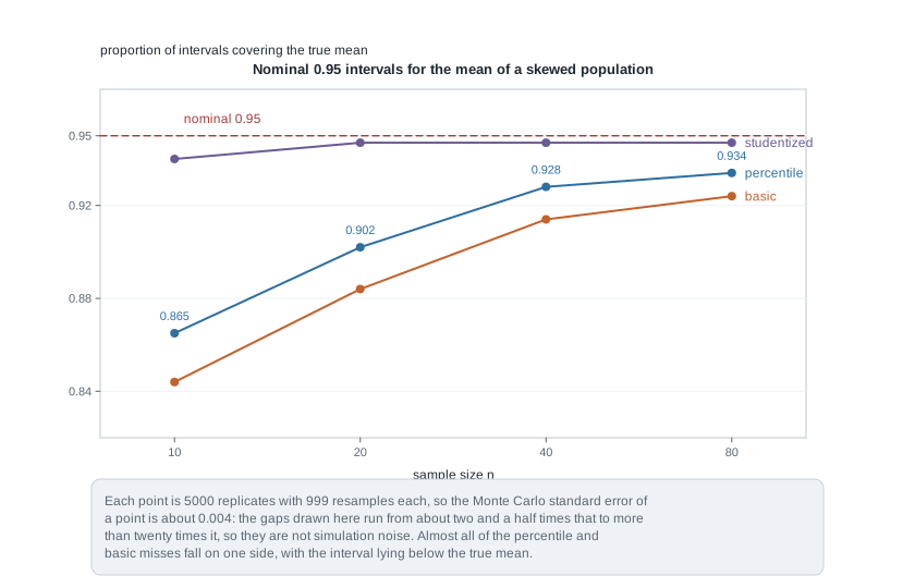
The numbers behind that plot are 0.865, 0.844 and 0.940 at \(n = 10\) for the percentile, basic and studentized intervals, and 0.934, 0.924 and 0.947 at \(n = 80\). Three readings matter. The studentized interval is close to nominal at every size, which is the Edgeworth result made visible. The other two undercover badly at small \(n\) and improve slowly, at the \(n^{-1/2}\) rate the theory predicts. And the misses are one-sided: at \(n = 10\) the percentile interval falls entirely below the true mean in 11.8 percent of replicates and entirely above in 1.7 percent, so calling it a symmetric statement about uncertainty misdescribes the error in both size and direction.
Each coverage number is itself an estimate. With \(R = 5000\) replicates and true coverage near 0.9 the Monte Carlo standard error is \(\sqrt{0.9 \times 0.1/5000} = 0.0042\), so differences of one hundredth are real and differences of one thousandth are not. Report that figure alongside any coverage study; without it the table cannot be read.
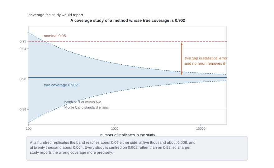
That is the two errors in one picture. The band reaches two Monte Carlo standard errors either side of a true coverage of 0.902, which is the percentile interval’s coverage at \(n = 20\) above: about 0.06 either side at a hundred replicates, 0.008 at five thousand, 0.004 at twenty thousand. The gap to 0.95 never enters the band. A bigger study reports the shortfall more precisely; only a bigger sample, or a better interval, removes it.
Where the bootstrap fails
Consistency is not automatic, and the instructive failures are the clean ones.
A non-smooth functional: the sample maximum. Let \(X_1, \dots, X_{10}\) be independent and uniform on the interval from \(0\) to \(\theta\), with \(\theta\) estimated by the sample maximum. Each resample draws from the observed values, so \(P^*(\hat\theta^* \le x_{(j)}) = (j/10)^{10}\) and the bootstrap distribution puts probability \(1 - (9/10)^{10} = 0.651\) on the single value \(x_{(10)}\). In general that atom is \(1 - (1 - 1/n)^n\), which tends to \(1 - e^{-1} = 0.632\) rather than vanishing, while the true sampling distribution of the maximum is continuous and puts probability zero on any one value.
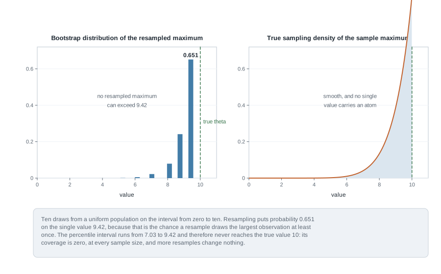
The consequence is not subtle. Every resampled maximum is at most the observed maximum, which is itself at most \(\theta\), so the percentile interval contains \(\theta\) with probability zero at every sample size. With the ten values \(1.31, 2.07, 3.42, 3.98, 5.25, 6.14, 7.03, 8.11, 8.76, 9.42\) drawn from a uniform population on the interval from \(0\) to \(10\), that interval runs from \(7.03\) to \(9.42\) and misses. The basic interval, which reflects, runs from \(9.42\) to \(11.81\) and does contain \(10\) — but its coverage is not 0.95 either: under the quantile convention fixed above it integrates in closed form to \(7/8\) at every sample size \(n \ge 9\), and to \(3/4\) at the smaller sizes \(n = 3\) through \(n = 8\). Reflection rescued the procedure from certain failure and left it miscalibrated.
Three further failures are worth naming. Under heavy tails the bootstrap for the sample mean is consistent when the population variance is finite and inconsistent when the population lies in the domain of attraction of a stable law with index below two, and no single data set reveals which case you are in. Under dependence, independent resampling destroys serial correlation, so the bootstrap distribution of a time-series mean understates its variance whenever the autocorrelations are positive; resampling contiguous blocks is the repair. At a boundary, if \(\theta\) sits on the edge of the parameter space the limiting distribution is not the smooth one the bootstrap reproduces — the failure that broke Wilks’ theorem in Week 5, in a resampling costume. One condition covers all four: the bootstrap is consistent when the functional is differentiable at \(F\) in an appropriate sense and the empirical process converges.
The misreading to avoid
The sentence to dismantle is this: the bootstrap gives the distribution of the parameter, so there is a 95 percent probability that the true ratio lies between 2.35 and 2.82, and if I want more accuracy I run more resamples. Three errors are packed into it.
What the distribution is. The histogram in the ratio example is the conditional law of \(\hat\theta^*\) given the observed data. It is centred at \(\hat\theta = 2.50\), not at \(\theta\), and it estimates the sampling variability of \(\hat\theta - \theta\); the resulting interval carries the repeated-sampling meaning Week 4 established, so coverage is a property of the procedure over hypothetical repetitions rather than of the one interval in front of you. A distribution for \(\theta\) given the data is a posterior, and a posterior requires a prior that no step here supplied.
Construction is not calibration. The derivation of the percentile interval guarantees 95 percent coverage only under a transformation assumption that may be false, and the coverage study is the check. Saying “95 percent” about a procedure that covers 87 percent of the time is a factual error about the procedure, not a matter of interpretation.
Buying the wrong thing. More resamples reduce simulation error, which was already small. They cannot touch the difference between \(\hat F_n\) and \(F\), and that difference is what a coverage shortfall is made of. The ratio example makes this vivid: its bootstrap distribution was computed exactly, so its simulation error was zero and its calibration problem unaffected. The companion slogan, that the bootstrap is assumption-free, is false for the same reason: it assumes an independent sample from one distribution, and a functional smooth enough there for the plug-in to converge at the usual rate.
Practice on your own
These are for self-checking as you read, not for submission.
- A derivation. Show that when the bootstrap distribution of \(\hat\theta^*\) is symmetric about \(\hat\theta\) the percentile and basic intervals coincide exactly, and that when it is right-skewed the basic interval extends further below \(\hat\theta\) than above. Say why that direction is the defensible one if you believe the pivot argument.
- An equivariance check. Prove that for strictly increasing \(m\) the percentile interval for \(m(\theta)\) is the image under \(m\) of the percentile interval for \(\theta\), then build a numerical counterexample showing the basic interval lacks this property.
- A jackknife by hand. For \(\theta = \mu^2\) estimated by \(\bar{x}^2\) the exact bias is \(\sigma^2/n\). Derive that, compute the jackknife bias estimate on the five lifetimes above, and check that it reproduces \(s^2/n\).
- A short simulation. Draw samples of size \(n\) from a uniform population and confirm that the exact bootstrap atom at the observed maximum approaches \(1 - e^{-1}\). Then estimate the coverage of the basic interval at \(n = 10\), compare with the exact \(7/8\) above, and report your Monte Carlo standard error.
- A condition to check. For the median, state which condition of the smooth function model fails, and why deleting blocks repairs the variance estimate when deleting one does not.
Where to read more
- The open graduate reference is MIT OpenCourseWare 18.655 Mathematical Statistics, whose treatment of asymptotic approximation goes past this page’s informal statements about differentiability of functionals.
- Penn State STAT 415 gives a gentler parallel treatment of interval estimation and simulation, useful if the inversion arguments moved too fast.
- The optional Hogg, McKean, and Craig alignment for this week is Chapter 4.8 through 4.9, on bootstrap and resampling procedures. That text is optional and never required to be purchased.
- Computing needs only the R Project for Statistical Computing and Quarto, both free; the enumeration above is one call to
expand.gridand one toapply. - Course pages: the notes overview, the syllabus, the schedule, and the resources page.
Where this goes next
Week 12 takes up procedures whose null distributions are known exactly without any resampling, because they depend only on ranks. The sign, signed-rank, and rank-sum tests get those distributions by counting arrangements, closer in spirit to Week 10 than to this week, and the comparison to draw is between a method exact under a weak assumption and one approximate under almost none. Watch the estimand: the rank-sum test does not estimate a difference in means unless a shift model holds, just as the bootstrap here estimates the sampling distribution of one functional and nothing else.
Carry two habits forward. Name the estimand as a functional before choosing a procedure, since most disagreements between methods are disagreements about the target rather than the arithmetic. And when a procedure claims a level or a coverage, ask what study established it and with what Monte Carlo standard error. Return to the previous unit, go on to the next unit, or step back to the notes overview.