Week 8 — Orthogonal complements, adjoints, and the four fundamental subspaces

Where this week starts

Week 7 leaned on a notation it never defined properly. It wrote \(U^{\perp}\) for the vectors orthogonal to a subspace \(U\), proved that \(v - P_U v\) lands in it, and used that to get the best-approximation theorem and the normal equations. What it did not do is treat \(U^{\perp}\) as an object with theorems of its own. That is the first half of this week: \(U^{\perp}\) is a subspace, it is a complement of \(U\), and — the part worth slowing down for — it is a complement that nobody chose.

Recall how badly that failed before the inner product arrived. In Week 1 a subspace had many complements and none was preferred; the line \(\operatorname{span}\{(1,0)\}\) in \(\mathbb{R}^2\) is complemented by the \(y\)-axis, by \(\operatorname{span}\{(1,1)\}\), and by infinitely many other lines. In Week 4 the same shapelessness reappeared as the observation that an isomorphism \(V \to F^n\) is exactly the data of an ordered basis. An inner product repairs this: each finite-dimensional subspace gets one distinguished complement, produced by the geometry rather than chosen.

The second half introduces the map that carries the rest of the course. Given \(T \colon V \to W\) between inner product spaces, the adjoint \(T^{*} \colon W \to V\) is defined by a single equation relating two inner products taken in two different spaces. It is not a symbol-shuffling operation on arrays; it becomes the conjugate transpose only after you agree to use orthonormal bases at both ends, and almost every error students make with adjoints traces back to dropping that clause. By the end the two halves meet: \(\ker T^{*}\) and \(\operatorname{im} T\) are orthogonal complements in \(W\), \(\operatorname{im} T^{*}\) and \(\ker T\) are orthogonal complements in \(V\), and those two sentences organise all four subspaces attached to a map into two complementary pairs — yielding, as a corollary rather than an appeal to row reduction, the theorem that row rank equals column rank.

Why this matters beyond the definition

Here is a claim that sounds harmless and is wrong. A linear system \(Ax = b\) has a solution set exactly when \(b\) avoids something special. The sharp criterion comes from this week: \(Ax = b\) is solvable exactly when \(b \perp \ker A^{\mathsf{T}}\), because \(\operatorname{im} A = (\ker A^{\mathsf{T}})^{\perp}\). That turns an existence question into finitely many inner products against a basis of \(\ker A^{\mathsf{T}}\), and it explains why a least-squares problem has a nonzero residual precisely when \(b\) has a component there.

The second stake bites in computation. A student who believes “the adjoint is the transpose” will write \(A^{\mathsf{T}}\) for an operator whose matrix was taken in a convenient but non-orthonormal basis, and will get a different operator entirely. The second worked example computes an adjoint whose matrix has entries \(-6\), \(-3\), \(12\), \(6\) while the original operator’s matrix has entries \(0\), \(1\), \(0\), \(0\). No amount of transposing turns one into the other.

What you will be able to do

• Prove that \(U^{\perp}\) is a subspace and that \(V = U \oplus U^{\perp}\) whenever \(U\) is finite-dimensional, naming where that hypothesis enters.
• Exhibit a subspace of an infinite-dimensional inner product space with \((U^{\perp})^{\perp} \ne U\), and a subspace over \(\mathbb{F}_2\) with \(U \cap U^{\perp} \ne \{0\}\).
• State and prove Riesz representation in finite dimensions, and use it to construct \(T^{*}\) with both existence and uniqueness.
• Compute the matrix of \(T^{*}\) in a general basis, and say why it reduces to the conjugate transpose exactly when the basis is orthonormal.
• Prove \(\ker T^{*} = (\operatorname{im} T)^{\perp}\) and \(\operatorname{im} T^{*} = (\ker T)^{\perp}\), and derive \(\operatorname{rank} T = \operatorname{rank} T^{*}\).
• Compute all four fundamental subspaces of an explicit real or complex matrix, with bases, verifying the relations by hand.

Terms and notation worth fixing

Symbol or term	What it means on this page
\(\langle u, v \rangle\)	linear in the first slot, conjugate-linear in the second, as fixed in Week 5
\(U^{\perp}\)	all \(v\) with \(\langle v, u \rangle = 0\) for every \(u \in U\); read “U perp”
\(P_U\)	orthogonal projection onto a finite-dimensional \(U\), from Week 7
\(T^{*}\)	the adjoint of \(T \colon V \to W\): a map \(W \to V\), defined by an inner product identity
\(A^{*}\)	conjugate transpose: transpose, then conjugate every entry
\(A^{\mathsf{T}}\)	plain transpose; equal to \(A^{*}\) over \(\mathbb{R}\), different over \(\mathbb{C}\)
\(G\), the Gram matrix	for an ordered basis \((u_1, \dots, u_n)\), the array with \(G_{ij} = \langle u_i, u_j \rangle\)
self-adjoint, unitary, orthogonal	\(T^{*} = T\); \(T^{*}T = TT^{*} = I\) over \(\mathbb{C}\); the same over \(\mathbb{R}\)

Throughout, \(F\) is \(\mathbb{R}\) or \(\mathbb{C}\) unless stated otherwise. That is not laziness: positive-definiteness needs an ordering on the scalars, and no finite field has one. The last subsection of the first half shows what breaks over \(\mathbb{F}_2\).

Orthogonal complements and the canonical splitting

Fix an inner product space \(V\) over \(F\) and a subset \(S \subseteq V\), and define \[S^{\perp} = \{ v \in V : \langle v, u \rangle = 0 \text{ for every } u \in S \}.\] Nothing asks \(S\) to be a subspace, and it is worth remembering that \(S^{\perp}\) is one even when \(S\) is a scrappy finite list. Orthogonality is symmetric even over \(\mathbb{C}\): conjugate symmetry gives \(\langle v, u \rangle = \overline{\langle u, v \rangle}\), and a complex number vanishes exactly when its conjugate does.

The complement a subspace comes with

Proposition. For any subset \(S\) of an inner product space \(V\), the set \(S^{\perp}\) is a subspace of \(V\), and \(S^{\perp} = \operatorname{span}(S)^{\perp}\).

Argument. Since \(\langle 0, u \rangle = 0\) for every \(u\), the set is nonempty. If \(x, y \in S^{\perp}\) and \(a \in F\), then for every \(u \in S\) linearity in the first slot gives \(\langle x + a y, u \rangle = \langle x, u \rangle + a \langle y, u \rangle = 0\), so the Week 1 subspace criterion applies. For the second claim, \(\operatorname{span}(S) \supseteq S\) forces \(\operatorname{span}(S)^{\perp} \subseteq S^{\perp}\); conversely, if \(v\) is orthogonal to \(u_1, \dots, u_k\) then conjugate-linearity in the second slot gives \(\langle v, \sum_i a_i u_i \rangle = \sum_i \overline{a_i}\,\langle v, u_i \rangle = 0\), and every member of the span is such a finite combination.

That second clause is why \(U^{\perp}\) is checkable in practice: you need only test a spanning set. Notice too that the proof used nothing but linearity in the first slot and conjugate-linearity in the second — no finite dimension, no positive-definiteness, no basis.

Theorem (orthogonal decomposition). Let \(V\) be an inner product space over \(F\) and let \(U \subseteq V\) be a finite-dimensional subspace. Then \(V = U \oplus U^{\perp}\): every \(v\) is \(u + x\) with \(u \in U\) and \(x \in U^{\perp}\), uniquely. The space \(V\) itself need not be finite-dimensional.

Argument. Since \(U\) is finite-dimensional, Gram-Schmidt (Week 6) turns any basis of \(U\) into an orthonormal basis \((e_1, \dots, e_m)\); this is the only place that hypothesis is used. Given \(v\), set \[u = P_U v = \sum_{i=1}^{m} \langle v, e_i \rangle e_i \in U, \qquad x = v - u .\] Linearity in the first slot and orthonormality give \(\langle u, e_j \rangle = \sum_i \langle v, e_i \rangle \langle e_i, e_j \rangle = \langle v, e_j \rangle\), so \(\langle x, e_j \rangle = 0\) for each \(j\); the proposition then puts \(x\) in \(U^{\perp}\). Hence \(U + U^{\perp} = V\). For directness, take \(y \in U \cap U^{\perp}\): it is orthogonal to every vector of \(U\) and lies in \(U\), so \(\langle y, y \rangle = 0\) and positive-definiteness forces \(y = 0\). By the Week 1 characterisation, \(U \cap U^{\perp} = \{0\}\) is exactly what makes the sum direct and the expression unique.

A vector resolved into its component in a subspace and its component in the orthogonal complement.

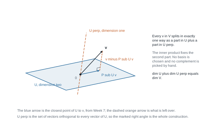
The picture is the theorem with the argument left visible: the blue arrow is \(P_U v\), the closest point of \(U\) to \(v\) from Week 7, the dashed orange arrow is \(v - P_U v\), and the marked right angle is the only property of it used. Notice what the picture lacks — a basis of the plane. Two orthonormal bases of \(U\) give the same \(P_U v\), since uniqueness pins both components down before any basis is named.

Say plainly what has changed since Week 1. There, a complement of \(U\) existed but was one of many, produced by extending a basis and depending on the extension. Here it is \(U^{\perp}\), determined by \(U\) and the inner product with no further choice — canonical relative to the inner product, a clause that matters, since a different inner product on the same \(V\) gives a different \(U^{\perp}\).

The dimension count and the double complement

Corollary. If \(V\) is finite-dimensional and \(U \subseteq V\) is a subspace, then \(\dim U + \dim U^{\perp} = \dim V\).

Argument. \(U\) is finite-dimensional inside a finite-dimensional space, so \(V = U \oplus U^{\perp}\), and the Week 2 dimension formula reads \(\dim V = \dim U + \dim U^{\perp} - \dim(U \cap U^{\perp})\) with the last term zero.

Theorem. Let \(U\) be a finite-dimensional subspace of an inner product space \(V\). Then \((U^{\perp})^{\perp} = U\).

Argument. One containment is free: \(u \in U\) is orthogonal to everything in \(U^{\perp}\) by definition and by symmetry of orthogonality, so \(u \in (U^{\perp})^{\perp}\). For the other, take \(v \in (U^{\perp})^{\perp}\) and write \(v = u + x\) with \(u \in U\), \(x \in U^{\perp}\). Then \(x = v - u\) is a difference of two members of \((U^{\perp})^{\perp}\) — \(v\) by assumption, \(u\) by the containment just proved — so \(x\) lies in both \(U^{\perp}\) and \((U^{\perp})^{\perp}\), giving \(\langle x, x \rangle = 0\) and \(x = 0\). Hence \(v = u \in U\).

That proof never mentioned \(\dim V\). Only \(U\) had to be finite-dimensional — sharper than the usual textbook version, and worth having, because the failure below turns on \(U\) being infinite-dimensional rather than on \(V\).

Where the splitting fails

Dropping finite-dimensionality of \(U\). Let \(V_0 \subseteq F^{\mathbb{N}}\) be the sequences with finitely many nonzero entries — the subspace Week 2 warned about, the one that \(\{e_1, e_2, \dots\}\) actually spans — with \(\langle x, y \rangle = \sum_{n \ge 1} x_n \overline{y_n}\), a finite sum for every pair. Take \(F = \mathbb{R}\) for readability. The rule \(\varphi(x) = \sum_{n \ge 1} x_n / n\) is also a finite sum, hence a linear functional, and \(\varphi(e_1) = 1\) so it is not zero. Put \(U = \ker \varphi\), a subspace with \(U \ne V_0\).

For \(i \ne j\) the vector \(i\,e_i - j\,e_j\) lies in \(U\), since \(\varphi\) sends it to \(i/i - j/j = 0\). If \(y \in U^{\perp}\) then \(\langle y, i e_i - j e_j \rangle = i\,y_i - j\,y_j = 0\), so \(n\,y_n\) is one number \(c\) for every \(n\) and \(y_n = c/n\). But \(y\) has finitely many nonzero entries, so \(c = 0\) and \(y = 0\). Therefore \(U^{\perp} = \{0\}\), whence \(U \oplus U^{\perp} = U \subsetneq V_0\) and \((U^{\perp})^{\perp} = V_0 \ne U\). Both theorems fail, and the only missing hypothesis is finite-dimensionality of \(U\).

Dropping the field. The definition of \(U^{\perp}\) needs only a bilinear form, so try \(\langle x, y \rangle = x_1y_1 + x_2y_2\) on \(\mathbb{F}_2^2\) with \(U = \operatorname{span}\{(1,1)\}\). A vector \((x, y)\) is orthogonal to \((1,1)\) exactly when \(x + y = 0\), that is when \(x = y\), so \(U^{\perp} = \{(0,0), (1,1)\} = U\). Then \(U \cap U^{\perp} = U \ne \{(0,0)\}\) and \(U + U^{\perp} = U \ne \mathbb{F}_2^2\): the sum is neither direct nor everything. The step that broke is positive-definiteness, since \((1,1)\) is nonzero and orthogonal to itself. The dimension count \(1 + 1 = 2\) nevertheless survives, since it follows from nondegeneracy alone — a warning that a correct dimension count is not evidence that a splitting exists.

The adjoint of a linear map

Let \(V\) and \(W\) be inner product spaces over the same \(F\) and \(T \colon V \to W\) linear. The adjoint is the map \(T^{*} \colon W \to V\) satisfying \[\langle Tv, w \rangle_W = \langle v, T^{*}w \rangle_V \qquad \text{for every } v \in V \text{ and every } w \in W .\] The subscripts are written once and then dropped: the left inner product is computed in \(W\), the right one in \(V\). Two things must be established before that display means anything — that such a map exists, and that only one satisfies the identity.

The defining identity of the adjoint, drawn as two inner products taken in two different spaces.

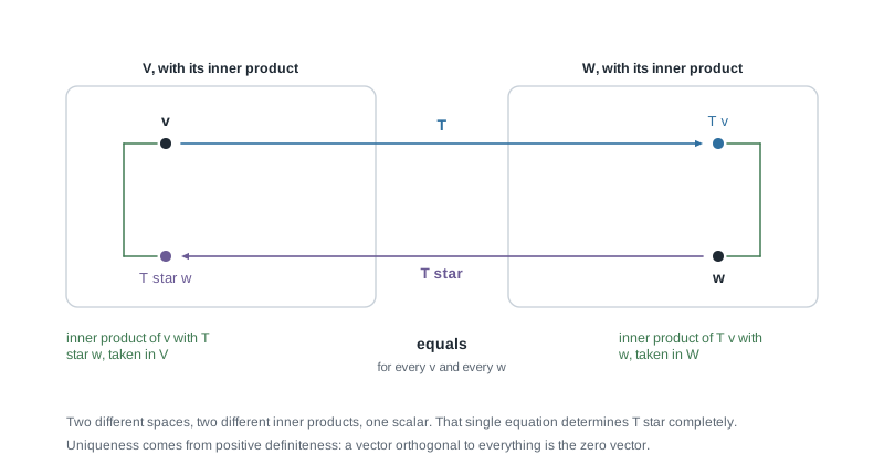
The figure separates the two sides so the asymmetry shows. On the right you push \(v\) forward through \(T\) and pair it with \(w\) in the codomain; on the left you pull \(w\) back through \(T^{*}\) and pair it with \(v\) in the domain. The two scalars agree, and nothing drawn is an array or names a basis.

Riesz representation, and the existence of the adjoint

Theorem (Riesz representation, finite-dimensional case). Let \(V\) be a finite-dimensional inner product space over \(F\) and \(\varphi \colon V \to F\) linear. Then there is exactly one \(w \in V\) with \(\varphi(v) = \langle v, w \rangle\) for all \(v\).

Argument. Finite-dimensionality lets Gram-Schmidt produce an orthonormal basis \((e_1, \dots, e_n)\). Set \(w = \sum_{j} \overline{\varphi(e_j)}\, e_j\). Week 6 expands \(v = \sum_i \langle v, e_i \rangle e_i\), so \[\langle v, w \rangle = \Big\langle \sum_i \langle v, e_i \rangle e_i , \sum_j \overline{\varphi(e_j)} e_j \Big\rangle = \sum_i \langle v, e_i \rangle\, \varphi(e_i) = \varphi(v),\] orthonormality killing the cross terms, conjugate-linearity in the second slot turning \(\overline{\varphi(e_j)}\) back into \(\varphi(e_j)\), and the last step being linearity of \(\varphi\) applied to the expansion of \(v\). If \(\langle v, w_1 \rangle = \langle v, w_2 \rangle\) for all \(v\), take \(v = w_1 - w_2\); positive-definiteness gives \(w_1 = w_2\).

Theorem (existence and uniqueness of the adjoint). Let \(V\) be finite-dimensional, \(W\) an inner product space over the same \(F\), and \(T \in \mathcal{L}(V, W)\). Then exactly one map \(T^{*} \colon W \to V\) satisfies \(\langle Tv, w \rangle = \langle v, T^{*}w \rangle\) for all \(v, w\), and it is linear.

Argument. Fix \(w\) and put \(\varphi_w(v) = \langle Tv, w \rangle\), linear in \(v\) because \(T\) is linear and the inner product is linear in its first slot. Riesz in \(V\) — legitimate because \(V\) is finite-dimensional — supplies a unique vector, named \(T^{*}w\), with \(\varphi_w(v) = \langle v, T^{*}w \rangle\) for all \(v\). Doing this for each \(w\) defines \(T^{*}\), and uniqueness of the Riesz vector is uniqueness of \(T^{*}\). Linearity is then a computation: for \(w_1, w_2 \in W\), \(a \in F\) and every \(v\), \[\langle v, T^{*}(w_1 + a w_2) \rangle = \langle Tv, w_1 \rangle + \overline{a}\,\langle Tv, w_2 \rangle = \langle v, T^{*}w_1 \rangle + \overline{a}\,\langle v, T^{*}w_2 \rangle = \langle v, T^{*}w_1 + a\,T^{*}w_2 \rangle,\] each conjugate appearing and then cancelling because the second slot is conjugate-linear, and uniqueness in Riesz finishes it. The two conjugations are what make \(T^{*}\) linear rather than conjugate-linear; they would not cancel under the opposite convention.

Four properties follow the same way — write the defining identity for the left-hand side, manipulate, invoke uniqueness — and are used below without comment: \((S + T)^{*} = S^{*} + T^{*}\), \((aT)^{*} = \overline{a}\,T^{*}\), \((T^{*})^{*} = T\), and \((S \circ T)^{*} = T^{*} \circ S^{*}\).

The matrix of the adjoint

Theorem. Let \(V\) and \(W\) be finite-dimensional inner product spaces over \(F\), let \(\mathcal{B} = (e_1, \dots, e_n)\) be an orthonormal ordered basis of \(V\) and \(\mathcal{C} = (f_1, \dots, f_m)\) an orthonormal ordered basis of \(W\), and let \(A = [T]_{\mathcal{C} \leftarrow \mathcal{B}}\). Then \([T^{*}]_{\mathcal{B} \leftarrow \mathcal{C}} = A^{*}\).

Argument. Orthonormality of \(\mathcal{C}\) lets Week 6 expand \(Te_j = \sum_i \langle Te_j, f_i \rangle f_i\), and the Week 4 definition makes the \(j\)-th column of \(A\) the coordinate column of \(Te_j\), so \(A_{ij} = \langle Te_j, f_i \rangle\). The same expansion in \(V\) gives \([T^{*}]_{\mathcal{B} \leftarrow \mathcal{C}}\) the entry \(\langle T^{*}f_i, e_j \rangle\) in row \(j\), column \(i\). Then \[\langle T^{*}f_i, e_j \rangle = \overline{\langle e_j, T^{*}f_i \rangle} = \overline{\langle Te_j, f_i \rangle} = \overline{A_{ij}} ,\] which is precisely the claim.

Every step used orthonormality; drop it and the conclusion is false, not merely unproved. Over \(\mathbb{R}\), for a general ordered basis \(\mathcal{B} = (u_1, \dots, u_n)\) of \(V\) with Gram matrix \(G_{ij} = \langle u_i, u_j \rangle\), the correct statement is \[[T^{*}]_{\mathcal{B} \leftarrow \mathcal{B}} = G^{-1}\, [T]_{\mathcal{B} \leftarrow \mathcal{B}}^{\mathsf{T}}\, G ,\] which reduces to the transpose exactly when \(G = I_n\), that is exactly when \(\mathcal{B}\) is orthonormal. To derive it, write \(A = [T]_{\mathcal{B}}\) and \(B = [T^{*}]_{\mathcal{B}}\) and expand both sides of \(\langle Tu_j, u_i \rangle = \langle u_j, T^{*}u_i \rangle\) in the basis: this reads \((GA)_{ij} = (GB)_{ji}\), so \(GA = (GB)^{\mathsf{T}} = B^{\mathsf{T}}G\) by symmetry of \(G\). Both worked examples check the formula against a direct computation.

Self-adjoint, unitary, and orthogonal maps

Three classes of operator on a finite-dimensional inner product space \(V\) are worth naming now, since Weeks 12 and 13 are about them.

Definition. \(T \in \mathcal{L}(V)\) is self-adjoint when \(T^{*} = T\), and unitary when \(T^{*}T = TT^{*} = I\). Over \(\mathbb{R}\) the conjugation does nothing and a unitary map is called orthogonal, with matrix condition \(A^{\mathsf{T}}A = I\).

Self-adjointness unpacks to \(\langle Tv, w \rangle = \langle v, Tw \rangle\) for all \(v, w\): the operator moves between slots at no cost. In an orthonormal basis its matrix satisfies \(A = A^{*}\), which over \(\mathbb{R}\) is symmetry.

Proposition. For \(T \in \mathcal{L}(V)\) with \(V\) finite-dimensional, these are equivalent: (i) \(T^{*}T = I\); (ii) \(\langle Tu, Tv \rangle = \langle u, v \rangle\) for all \(u, v\); (iii) \(\lVert Tv \rVert = \lVert v \rVert\) for all \(v\).

Argument. (i) gives (ii) since \(\langle Tu, Tv \rangle = \langle u, T^{*}Tv \rangle\). (ii) gives (iii) by taking \(u = v\) and square roots. (iii) gives (ii) by polarisation, which recovers the inner product from the norm — over \(\mathbb{R}\), \(\langle u, v \rangle = \tfrac{1}{2}(\lVert u + v \rVert^2 - \lVert u \rVert^2 - \lVert v \rVert^2)\), an identity needing \(2\) invertible, so the field matters here too. (ii) gives (i) because \(\langle u, (T^{*}T - I)v \rangle = 0\) for all \(u\) forces \((T^{*}T - I)v = 0\).

Finite-dimensionality is what upgrades \(T^{*}T = I\) to \(TT^{*} = I\): the first makes \(T\) injective, and an injective operator on a finite-dimensional space is surjective by rank-nullity from Week 3. On \(V_0\) the two conditions genuinely differ — the right shift preserves norms and has \(T^{*}T = I\), while \(TT^{*}\) is the projection killing the first coordinate.

Adjoint, self-adjoint, unitary, and orthogonal, each with its defining condition and its hypothesis.

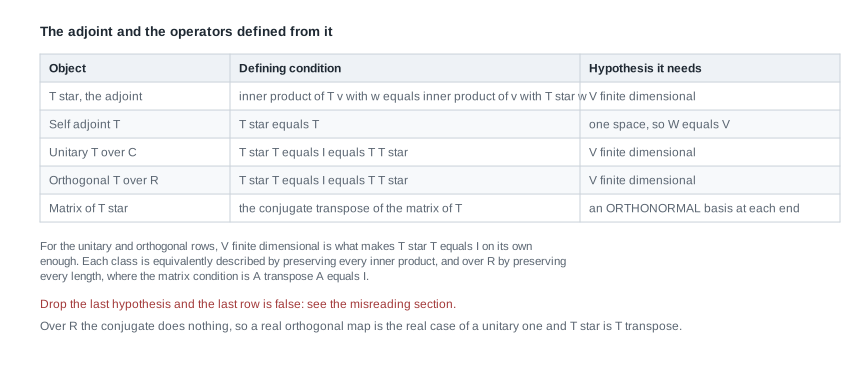
The table collects the four defining conditions with the hypothesis each needs beside it, and records beneath them the equivalent inner-product and norm characterisations of the unitary and orthogonal rows. Memorise the last row with its condition attached: the matrix of \(T^{*}\) is the conjugate transpose of the matrix of \(T\), relative to an orthonormal basis at each end. Strip that clause and you have the misreading this page ends with.

The four fundamental subspaces

A map carries four subspaces with it: \(\ker T\) and \(\operatorname{im} T^{*}\) inside \(V\), and \(\operatorname{im} T\) and \(\ker T^{*}\) inside \(W\). Week 3 produced two of them and related their dimensions; the adjoint produces the other two and relates all four by orthogonality. Here \(V\) and \(W\) are finite-dimensional inner product spaces over the same \(F\), with \(\dim V = n\), \(\dim W = m\), \(\operatorname{rank} T = r\).

Theorem. \(\ker T^{*} = (\operatorname{im} T)^{\perp}\) and \(\operatorname{im} T^{*} = (\ker T)^{\perp}\).

Argument. For the first, \(w \in \ker T^{*}\) means \(T^{*}w = 0\), which by positive-definiteness holds exactly when \(\langle v, T^{*}w \rangle = 0\) for every \(v\) — one direction immediate, the other by taking \(v = T^{*}w\). The defining identity rewrites that as \(\langle Tv, w \rangle = 0\) for every \(v\), which says \(w\) is orthogonal to every vector of \(\operatorname{im} T\). For the second, apply the first relation to \(T^{*}\), using \((T^{*})^{*} = T\): it reads \(\ker T = (\operatorname{im} T^{*})^{\perp}\). Take complements of both sides; the right becomes \(\operatorname{im} T^{*}\) by the double-complement theorem, which applies because \(\operatorname{im} T^{*}\) is a subspace of the finite-dimensional \(V\).

Corollary. \(\operatorname{rank} T = \operatorname{rank} T^{*}\).

Argument. \(\operatorname{rank} T^{*} = \dim (\ker T)^{\perp} = \dim V - \dim \ker T\) by the dimension corollary, and rank-nullity from Week 3 identifies that with \(\operatorname{rank} T\).

The four fundamental subspaces as two pairs of orthogonal complements, joined by the map and its adjoint.

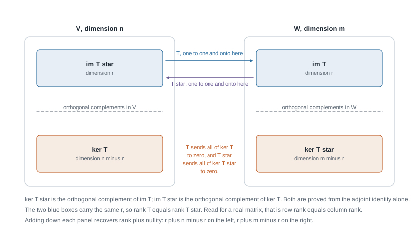
Read the figure’s claims off one at a time. Each panel is split by a dashed line into an orthogonal pair, so adding the dimensions in a panel returns \(n\) on the left and \(m\) on the right — rank-nullity for \(T\) and for \(T^{*}\). The two blue boxes carry the same \(r\), which is the corollary. The arrows record what the proofs give for free: \(T\) restricted to \(\operatorname{im} T^{*} = (\ker T)^{\perp}\) is injective, since a vector of that subspace killed by \(T\) lies in \(\ker T \cap (\ker T)^{\perp} = \{0\}\), and onto \(\operatorname{im} T\) because \(V = \ker T \oplus (\ker T)^{\perp}\) and the kernel part contributes nothing. So every such map is an isomorphism between one distinguished \(r\)-dimensional subspace of \(V\) and one of \(W\), flanked by two kernels.

Row rank equals column rank

Specialise to \(V = F^n\) and \(W = F^m\) with their standard inner products and \(T\) given by an \(m \times n\) matrix \(A\). The standard bases are orthonormal, so \(T^{*}\) is \(A^{*}\) and the corollary reads \(\operatorname{rank} A = \operatorname{rank} A^{*}\). Over \(\mathbb{R}\), \(A^{*} = A^{\mathsf{T}}\), whose column space is the row space of \(A\): the row rank of a real matrix equals its column rank. Over \(\mathbb{C}\) the same argument applies, and since conjugating every entry is a bijection preserving linear relations, \(\operatorname{rank} A^{*} = \operatorname{rank} A^{\mathsf{T}}\) as well.

You knew this as an undergraduate fact about row reduction, and Week 4 used it silently when treating rank as a property of the map. It is now proved, with no elimination anywhere — only the adjoint identity, positive-definiteness, and the dimension count. The cost is that \(F\) must be \(\mathbb{R}\) or \(\mathbb{C}\): row rank equals column rank over \(\mathbb{F}_2\) too, but this proof cannot reach it, and the \(\mathbb{F}_2\) example above shows why no repair through the standard bilinear form is available.

Worked example — the four subspaces of a three by two real matrix

Work in \(\mathbb{R}^n\) with the standard dot product, and let \[A = \begin{pmatrix} 1 & 1 \\ 1 & -1 \\ 1 & 0 \end{pmatrix}, \qquad T \colon \mathbb{R}^2 \to \mathbb{R}^3, \quad Tx = Ax .\] The standard bases are orthonormal and the entries real, so \(T^{*}\) is given by \(A^{\mathsf{T}}\). Find bases for all four subspaces, check both orthogonality relations by direct inner products, and check both dimension identities against Week 3.

Step 1. The image of \(T\). The columns \(c_1 = (1,1,1)^{\mathsf{T}}\) and \(c_2 = (1,-1,0)^{\mathsf{T}}\) are not proportional, so \(\operatorname{im} T = \operatorname{span}\{c_1, c_2\}\) has dimension \(r = 2\). A bonus: \(c_1 \cdot c_2 = 1 - 1 + 0 = 0\), so this basis of the image is already orthogonal.

Step 2. The kernel of \(T\). Independent columns mean \(Ax = 0\) forces \(x = 0\), so \(\ker T = \{0\}\) and \(\dim \ker T = 0\). Rank-nullity checks: \(2 + 0 = 2 = \dim \mathbb{R}^2\).

Step 3. The kernel of \(T^{*}\). With \(A^{\mathsf{T}} = \begin{pmatrix} 1 & 1 & 1 \\ 1 & -1 & 0 \end{pmatrix}\), solve \(y_1 + y_2 + y_3 = 0\) and \(y_1 - y_2 = 0\). The second gives \(y_2 = y_1\), and then \(y_3 = -2y_1\), so \(\ker T^{*} = \operatorname{span}\{(1, 1, -2)^{\mathsf{T}}\}\), of dimension \(1\).

Step 4. The image of \(T^{*}\). The columns of \(A^{\mathsf{T}}\) are \((1,1)^{\mathsf{T}}\), \((1,-1)^{\mathsf{T}}\), \((1,0)^{\mathsf{T}}\); the first two are independent, so \(\operatorname{im} T^{*} = \mathbb{R}^2\), of dimension \(2\). Rank-nullity for \(T^{*}\): \(2 + 1 = 3 = \dim \mathbb{R}^3\).

Step 5. Verify the relations. Test the spanning vector of \(\ker T^{*}\) against both columns: \[(1,1,-2) \cdot (1,1,1) = 1 + 1 - 2 = 0, \qquad (1,1,-2) \cdot (1,-1,0) = 1 - 1 + 0 = 0 .\] So \(\ker T^{*} \subseteq (\operatorname{im} T)^{\perp}\), and the dimensions agree at \(3 - 2 = 1\), so the containment is equality by Week 2. The second relation reads \(\operatorname{im} T^{*} = (\ker T)^{\perp}\), and here \(\ker T = \{0\}\) has complement all of \(\mathbb{R}^2\), matching Step 4. Both dimension identities hold, \(2 + 1 = 3\) and \(2 + 0 = 2\), and \(\operatorname{rank} T = \operatorname{rank} T^{*} = 2\).

Step 6. Split a vector. Because the columns are orthogonal the projection is easy by hand. Take \(b = (0,0,6)^{\mathsf{T}}\), with \(\lVert c_1 \rVert^2 = 3\) and \(\lVert c_2 \rVert^2 = 2\): \[P_U b = \frac{b \cdot c_1}{3}\,c_1 + \frac{b \cdot c_2}{2}\,c_2 = 2\,(1,1,1)^{\mathsf{T}} + 0\,(1,-1,0)^{\mathsf{T}} = (2,2,2)^{\mathsf{T}} .\] The residual is \(b - P_U b = (-2,-2,4)^{\mathsf{T}} = -2\,(1,1,-2)^{\mathsf{T}}\), a multiple of the basis vector from Step 3. That is the decomposition theorem in numbers: \(\mathbb{R}^3 = \operatorname{im} T \oplus \ker T^{*}\), with no other splitting available.

What this establishes: the four subspaces of this \(A\), their bases, and both relations, checked arithmetically. What it does not: anything about dependent columns. With two columns in \(\mathbb{R}^3\) the only way to make \(\ker T\) nonzero is to drop the rank to one. For \(A' = \begin{pmatrix} 1 & 2 \\ 1 & 2 \\ 1 & 2 \end{pmatrix}\) we get \(\ker T' = \operatorname{span}\{(2,-1)^{\mathsf{T}}\}\), \(\operatorname{im} T' = \operatorname{span}\{(1,1,1)^{\mathsf{T}}\}\), \(\operatorname{im} (T')^{*} = \operatorname{span}\{(1,2)^{\mathsf{T}}\}\), and \(\ker (T')^{*}\) the plane \(y_1 + y_2 + y_3 = 0\). Check the second relation there: \((1,2) \cdot (2,-1) = 2 - 2 = 0\), and \(2 - 1 = 1\) is the right dimension.

The same reasoning, transferred

Run the same questions over \(\mathbb{C}\), where the conjugate has somewhere to go. Let \[A = \begin{pmatrix} 1 & i \\ -i & 1 \end{pmatrix}, \qquad T \colon \mathbb{C}^2 \to \mathbb{C}^2 ,\] with \(\langle u, v \rangle = u_1\overline{v_1} + u_2\overline{v_2}\). First, \(A^{*} = A\): transposing gives \(\begin{pmatrix} 1 & -i \\ i & 1 \end{pmatrix}\) and conjugating returns \(A\). So \(T\) is self-adjoint, and the standard basis is orthonormal, so the matrix theorem applies.

The determinant is \(1 \cdot 1 - i \cdot (-i) = 1 - 1 = 0\), so \(r = 1\). The first row gives \(\ker T\) from \(x + iy = 0\), so \(\ker T = \operatorname{span}\{(-i, 1)\}\); the second row confirms it, since \((-i)(-i) + 1 = -1 + 1 = 0\). The columns are \((1, -i)\) and \((i, 1) = i\,(1, -i)\), so \(\operatorname{im} T = \operatorname{span}\{(1,-i)\}\). Since \(T^{*} = T\) the other two subspaces are these same two, and the relations become checkable identities: \[\langle (-i, 1), (1, -i) \rangle = (-i)\overline{1} + 1 \cdot \overline{(-i)} = -i + i = 0 .\] So \(\ker T^{*} = (\operatorname{im} T)^{\perp}\), both sides one-dimensional in a two-dimensional space, and \(\operatorname{im} T^{*} = (\ker T)^{\perp}\) by the same computation read backwards. Dimensions: \(1 + 1 = 2\) on both sides, with \(\operatorname{rank} T = \operatorname{rank} T^{*} = 1\).

Now the part only \(\mathbb{C}\) can show. Use the plain transpose: \(A^{\mathsf{T}} = \begin{pmatrix} 1 & -i \\ i & 1 \end{pmatrix}\), whose kernel comes from \(x - iy = 0\), giving \(\operatorname{span}\{(i, 1)\}\). Is that \((\operatorname{im} T)^{\perp}\)? Compute \(\langle (i,1), (1,-i) \rangle = i + 1 \cdot \overline{(-i)} = i + i = 2i \ne 0\). It is not. What stayed the same: the definitions, the two relations, the dimension bookkeeping, and testing orthogonality against a spanning set. What changed: the conjugate is no longer invisible, and \(A^{\mathsf{T}}\) where \(A^{*}\) belongs produces a subspace failing the theorem by a clean \(2i\).

Second worked example — the adjoint of differentiation on linear polynomials

Nothing so far required \(T\) to be a matrix. Take \(V = P_1(\mathbb{R})\), the real polynomials of degree at most one, so \(\dim V = 2\) with ordered basis \(\mathcal{B} = (1, x)\), and give it the inner product \(\langle f, g \rangle = \int_0^1 f(t)g(t)\,dt\) from Week 5. Let \(D\) be differentiation, \(D(a + bx) = b\), which maps \(V\) into \(V\).

Step 1. The Gram matrix. The three integrals needed are \(\langle 1, 1 \rangle = 1\), \(\langle 1, x \rangle = \tfrac12\), and \(\langle x, x \rangle = \tfrac13\), so \[G = \begin{pmatrix} 1 & \tfrac12 \\ \tfrac12 & \tfrac13 \end{pmatrix}, \qquad \det G = \tfrac13 - \tfrac14 = \tfrac1{12}, \qquad G^{-1} = \begin{pmatrix} 4 & -6 \\ -6 & 12 \end{pmatrix} .\] Confirm the inverse: the entries of \(G\,G^{-1}\) are \(4 - 3 = 1\), \(-6 + 6 = 0\), \(2 - 2 = 0\), and \(-3 + 4 = 1\). Since \(G \ne I_2\), the basis \(\mathcal{B}\) is not orthonormal.

Step 2. Solve for \(D^{*}g\) directly. Write \(g = a + bx\) and look for \(D^{*}g = c + dx\). The identity must hold for every \(f\), and by linearity it suffices to impose it for \(f = 1\) and \(f = x\). With \(f = 1\): \(D(1) = 0\), so the left side is \(0\) and the right side is \(\langle 1, c + dx \rangle = c + \tfrac{d}{2}\), giving \(c + \tfrac{d}{2} = 0\). With \(f = x\): \(D(x) = 1\), so the left side is \(\langle 1, a + bx \rangle = a + \tfrac{b}{2}\) and the right side is \(\langle x, c + dx \rangle = \tfrac{c}{2} + \tfrac{d}{3}\). From the first, \(c = -\tfrac{d}{2}\); substituting, \(-\tfrac{d}{4} + \tfrac{d}{3} = \tfrac{d}{12} = a + \tfrac{b}{2}\), so \(d = 12a + 6b\) and \(c = -6a - 3b\). Therefore \[D^{*}(a + bx) = (-6a - 3b) + (12a + 6b)\,x, \qquad D^{*}(1) = -6 + 12x, \qquad D^{*}(x) = -3 + 6x .\]

Step 3. Compare the two matrices. Reading off columns, \([D]_{\mathcal{B}} = \begin{pmatrix} 0 & 1 \\ 0 & 0 \end{pmatrix}\) and \([D^{*}]_{\mathcal{B}} = \begin{pmatrix} -6 & -3 \\ 12 & 6 \end{pmatrix}\). The transpose of the first is \(\begin{pmatrix} 0 & 0 \\ 1 & 0 \end{pmatrix}\), which is not the second and does not resemble it. The Gram formula reconciles them: \[G^{-1} [D]_{\mathcal{B}}^{\mathsf{T}} G = \begin{pmatrix} 4 & -6 \\ -6 & 12 \end{pmatrix} \begin{pmatrix} 0 & 0 \\ 1 & \tfrac12 \end{pmatrix} = \begin{pmatrix} -6 & -3 \\ 12 & 6 \end{pmatrix} ,\] where the product \([D]_{\mathcal{B}}^{\mathsf{T}} G = \begin{pmatrix} 0 & 0 \\ 1 & \tfrac12 \end{pmatrix}\) was formed first.

Step 4. Two independent checks. Test the identity on \(f = x\), \(g = 1\): the left side is \(\langle Dx, 1 \rangle = \langle 1, 1 \rangle = 1\) and the right side is \(\langle x, -6 + 12x \rangle = -6 \cdot \tfrac12 + 12 \cdot \tfrac13 = -3 + 4 = 1\). Test \(f = g = x\): the left side is \(\langle 1, x \rangle = \tfrac12\) and the right side is \(\langle x, -3 + 6x \rangle = -\tfrac32 + 2 = \tfrac12\). Next, \(D^2 = 0\) on \(P_1(\mathbb{R})\) and \((D^2)^{*} = (D^{*})^2\), so \([D^{*}]_{\mathcal{B}}^2\) must vanish; its entries are \(36 - 36\), \(18 - 18\), \(-72 + 72\), and \(-36 + 36\). It does.

Step 5. What the arithmetic says. Integration by parts explains the numbers: for \(f, g \in P_1(\mathbb{R})\), \(\langle Df, g \rangle = f(1)g(1) - f(0)g(0) - \langle f, Dg \rangle\), so \(D^{*}\) is \(-D\) plus a correction carrying the boundary terms, and those terms are what stop \(D^{*}\) from being the tidy \(-D\). Note also \(\operatorname{rank} D = \operatorname{rank} D^{*} = 1\), the columns of \([D^{*}]_{\mathcal{B}}\) being proportional — this week’s corollary, on an operator with no matrix of its own until a basis was picked.

The misreading to avoid

The misreading: the adjoint is the transpose, so I can compute \(T^{*}\) by transposing whatever matrix I happen to have written down. The smallest counterexample fits in three lines and is worth carrying.

Work in \(\mathbb{R}^2\) with the dot product and let \(T\) be the swap, \(T(x_1, x_2) = (x_2, x_1)\). Its standard matrix is symmetric, and \(\langle Tu, v \rangle = u_2v_1 + u_1v_2 = \langle u, Tv \rangle\), so \(T\) is self-adjoint and \(T^{*} = T\) as maps. Take \(\mathcal{B} = (b_1, b_2)\) with \(b_1 = (1,0)\) and \(b_2 = (1,1)\) — legal, and not orthonormal. Then \(Tb_1 = (0,1) = -b_1 + b_2\) and \(Tb_2 = (1,1) = b_2\), so \[[T]_{\mathcal{B} \leftarrow \mathcal{B}} = \begin{pmatrix} -1 & 0 \\ 1 & 1 \end{pmatrix} = [T^{*}]_{\mathcal{B} \leftarrow \mathcal{B}} ,\] the two being equal because \(T^{*} = T\). But the transpose of that array is \(\begin{pmatrix} -1 & 1 \\ 0 & 1 \end{pmatrix}\), a different matrix. In this basis the matrix of the adjoint is not the transpose of the matrix of the map. The Gram matrix is \(G = \begin{pmatrix} 1 & 1 \\ 1 & 2 \end{pmatrix}\) with \(\det G = 1\) and \(G^{-1} = \begin{pmatrix} 2 & -1 \\ -1 & 1 \end{pmatrix}\); the formula gives \([T]^{\mathsf{T}}G = \begin{pmatrix} 0 & 1 \\ 1 & 2 \end{pmatrix}\) and then \(G^{-1}\begin{pmatrix} 0 & 1 \\ 1 & 2 \end{pmatrix} = \begin{pmatrix} -1 & 0 \\ 1 & 1 \end{pmatrix}\), recovering \([T^{*}]_{\mathcal{B}}\).

Where the misreading comes from is worth naming. Undergraduate linear algebra works in \(\mathbb{R}^n\) with the standard basis nearly always, and that basis is orthonormal, so the hypothesis is satisfied silently every time and never announces itself. The corrective is a question to ask before transposing anything: is the basis I am using orthonormal? If \(G \ne I\), transposing computes another operator, the one with matrix \(G [T^{*}]_{\mathcal{B}} G^{-1}\).

A second misreading is the same error in different clothes: \(U^{\perp}\) is a complement of \(U\), so every complement of \(U\) is orthogonal to it. No. In \(\mathbb{R}^2\) the line \(\operatorname{span}\{(1,0)\}\) has \(\operatorname{span}\{(1,1)\}\) as a complement, the lines being distinct with dimensions summing to two, yet \((1,0) \cdot (1,1) = 1 \ne 0\). Being a complement is a statement about sums and intersections; being the orthogonal complement is a statement about the inner product, and is strictly stronger.

Practice on your own

These are for your own checking rather than for submission, and all are within reach of Weeks 1 through 8.

1. Complements of a plane. In \(\mathbb{R}^4\) with the dot product, let \(U = \operatorname{span}\{(1,1,0,0), (0,0,1,1)\}\). Find a basis of \(U^{\perp}\), verify \(\dim U + \dim U^{\perp} = 4\), then exhibit a complement of \(U\) that is not \(U^{\perp}\), proving it is a complement and computing one nonzero inner product that shows it is not orthogonal to \(U\).
2. An adjoint on matrices. Let \(V = M_2(\mathbb{R})\) with \(\langle A, B \rangle = \operatorname{tr}(B^{\mathsf{T}}A)\), and check first that this is an inner product. Fix \(M \in V\) and let \(T(A) = MA\). Prove \(T^{*}(A) = M^{\mathsf{T}}A\) from the defining identity and the cyclic property of the trace, then decide for which \(M\) the operator \(T\) is self-adjoint.
3. Solvability by orthogonality. For the \(A\) of the first worked example, decide which of \((1,1,1)^{\mathsf{T}}\), \((1,0,0)^{\mathsf{T}}\), and \((3,1,2)^{\mathsf{T}}\) lie in \(\operatorname{im} T\), using only inner products against the basis of \(\ker T^{*}\) from Step 3. For each failure compute the residual and confirm it is a multiple of \((1,1,-2)^{\mathsf{T}}\).
4. The hypothesis in the double complement. Prove \(U \subseteq (U^{\perp})^{\perp}\) for every subspace of every inner product space, with no finiteness assumed. Then locate the exact sentence in this page’s proof of equality that fails for \(U = \ker \varphi\) inside \(V_0\).
5. Unitary from orthonormal bases. Let \(V\) be finite-dimensional over \(\mathbb{C}\) and let \(T \in \mathcal{L}(V)\) carry some orthonormal basis to an orthonormal basis. Prove \(T\) is unitary. Then decide whether the conclusion survives when “basis” is weakened to “independent set of the right size”, with a counterexample if it does not.

Where to read more

A second treatment in a different voice is often what makes a theorem settle. The three addresses below are offered online at no cost by their providers; availability and licence terms are as those providers state them, and neither is confirmed here.

• MIT OpenCourseWare 18.700 Linear Algebra — a proof-based course whose treatment of inner product spaces, orthogonal complements, and adjoints runs parallel to this week.
• Linear Algebra Done Wrong by Sergei Treil — develops the adjoint from the inner product rather than from the transpose, and is careful about the orthonormality hypothesis.
• MIT OpenCourseWare 18.06 Linear Algebra — the computational complement, and the source of the four-subspaces framing, exercised on explicit numerical arrays.
• The optional Roman alignment for this week is the chapter on inner product spaces, in the sections on orthogonal projections and on the adjoint of a linear map. That text is an optional reference: a borrowed or library copy suffices, purchase is not required for anything here, and nothing from it is reproduced or adapted on this page.
• Course pages: the notes overview, the syllabus, the schedule, and the resources page. The learning management system remains authoritative for section logistics and graded details.

Where this goes next

The adjoint is the hinge between the geometric half of the course and the spectral half. Everything in Weeks 12 and 13 — the spectral theorem for self-adjoint operators, normal operators, the unitary diagonalisation of Hermitian matrices — is a statement about how \(T\) and \(T^{*}\) interact. Keep two things at hand: the identity \(\langle Tv, w \rangle = \langle v, T^{*}w \rangle\), which is the definition and the proof technique at once, and the splitting \(V = U \oplus U^{\perp}\), which lets an invariant subspace be peeled off without disturbing what remains.

Week 9, on bilinear forms, quadratic forms, congruence, and inertia, closes the inner-product block by asking what survives when positive-definiteness is dropped. That is the hypothesis whose failure over \(\mathbb{F}_2\) broke the splitting earlier on this page, so the question is already on the table: without it \(U \cap U^{\perp}\) can be nonzero, and Sylvester’s law of inertia replaces the orthogonal decomposition. To look back instead: Week 7 supplies the projection \(P_U\) and the best-approximation theorem used here, Week 6 supplies the orthonormal bases every proof quietly depended on, and Week 3 supplies rank-nullity. The notes index and the course home page list what is available.