Week 3 — Linear transformations, kernel and image, and rank-nullity

Where this week starts

Weeks 1 and 2 were about one space at a time. Week 1 gave you the objects — a vector space over a field \(F\), its subspaces, the difference between a sum and a direct sum. Week 2 gave you the tape measure: independence, bases, and the theorem that any two bases of a finitely generated space have the same size, so \(\dim V\) belongs to the space and not to whoever chose the basis. All of it was internal. Nothing yet related two different spaces, which is a strange gap, because the object your undergraduate course spent a semester on — the matrix — exists precisely to relate two spaces.

This week closes the gap. A linear transformation \(T \colon V \to W\) is a function between vector spaces over the same field that respects the two operations, and that is the whole definition. From it comes a surprising amount. The first surprise is how little data a linear map carries: choose a basis of \(V\), say where each basis vector goes, and the map is determined, with no compatibility condition on your choices. The second is that the two ways a map can fail to be a bijection — failing to be injective, failing to be surjective — are not independent defects. In finite dimensions they are two halves of one dimension count, the rank-nullity theorem, whose content is that the size of what \(T\) crushes and the size of what \(T\) reaches must add up to the size of where \(T\) started.

The week’s third job is to explain why that count is inevitable rather than lucky. The direct proof extends a basis of \(\ker T\) to a basis of \(V\) and checks that the added vectors map to a basis of \(\operatorname{im} T\). It is a good proof, but it leaves the theorem looking like an accident of basis-chasing. The quotient construction removes the impression: you build a space \(V / \ker T\) whose vectors are the cosets of \(\ker T\) — the sets of inputs \(T\) cannot tell apart — and the first isomorphism theorem gives \(V / \ker T \cong \operatorname{im} T\). Rank-nullity then follows in two lines.

By Friday, “linear map” should feel like the primary object and “matrix” like a derived one, the kernel should be the first thing you compute about any map, and “quotient space” should name something concrete: for \(\mathbb{R}^3\) modulo the \(z\)-axis, a family of parallel vertical lines. Week 4 chooses bases and turns \(T\) into a matrix; this week deliberately does not.

Why this matters beyond the definition

Here is a claim a well-trained undergraduate makes without hesitating. A homogeneous system of three equations in four unknowns has more unknowns than equations, so it has a nontrivial solution; three of the four degrees of freedom are used by the equations, so the solution set is a line. The first half is right, and rank-nullity is the reason. The second half is wrong, and rank-nullity is also the reason: it gives \(\operatorname{null} T = 4 - \operatorname{rank} T\) with \(\operatorname{rank} T \le 3\), so the kernel has dimension at least one. It is exactly one only when the three equations are genuinely independent, which nothing in the shape of the system guarantees.

The second stake concerns inhomogeneous systems. Ask whether the set of vectors satisfying \(Ax = b\) forms a subspace and you often get a yes, since the set satisfying \(Ax = 0\) certainly does. It does not, unless \(b = 0\): it is a coset \(x_0 + \ker A\), a translate of a subspace. Quotients are exactly the machinery for treating translates of subspaces as objects, which is why the second half of this page is not a digression.

What you will be able to do

• State the definition of a linear transformation and decide, with proof, whether a given function between concrete spaces is one — including a function that is additive but not homogeneous.
• Prove that a linear map is determined by its values on a basis, in both directions: arbitrary targets extend to a linear map, and two linear maps agreeing on a basis are equal.
• Prove that \(\ker T\) and \(\operatorname{im} T\) are subspaces, that \(T\) is injective exactly when \(\ker T = \{0\}\), and rank-nullity for finite-dimensional \(V\), naming where that hypothesis is used.
• Construct the quotient \(V / U\), verify its operations are well defined on representatives, and compute \(\dim (V/U)\) for finite-dimensional \(V\).
• Compute rank, nullity, kernel and image for differentiation on polynomials and for an explicit \(3 \times 4\) matrix, and track how the counts move when the characteristic changes.
• Exhibit a counterexample showing that the finite-dimensional consequences of rank-nullity fail without finite-dimensionality of \(V\) — in particular that an injective operator on \(F^{\mathbb{N}}\) need not be surjective — and one showing a map from a four-dimensional space to a three-dimensional space need not have a one-dimensional kernel.

Terms and notation worth fixing

Symbol or term	What it means in this course
\(T \colon V \to W\)	a linear map; \(V\) and \(W\) are spaces over the same field \(F\)
\(\ker T\)	\(\{ v \in V : Tv = 0 \}\), a subspace of the domain \(V\)
\(\operatorname{im} T\)	\(\{ Tv : v \in V \}\), a subspace of the codomain \(W\)
\(\operatorname{rank} T\), \(\operatorname{null} T\)	\(\dim \operatorname{im} T\) and \(\dim \ker T\)
\(\mathcal{L}(V, W)\)	all linear maps \(V \to W\), a space over \(F\) under pointwise operations
\(v + U\)	the coset \(\{ v + u : u \in U \}\): a subset of \(V\), a single element of \(V/U\)
\(V / U\)	the quotient space, whose elements are the cosets of \(U\)
\(\pi \colon V \to V/U\)	the canonical projection \(\pi(v) = v + U\), always linear and surjective

One convention to state once: \(T\) and \(S\) are reserved for maps throughout this block, and subspaces are \(U\), \(X\), \(Y\). That matters more this week than last, because kernels and images are subspaces attached to a map, and the letter should always tell you which kind of object you are holding.

Linear maps and how little determines them

A function between vector spaces is a loose thing; a linear one is rigid to the point of carrying almost no information. This section makes both halves precise.

Additivity, homogeneity, and two functions that fail

Definition. Let \(V\) and \(W\) be vector spaces over the same field \(F\). A function \(T \colon V \to W\) is a linear transformation if for all \(u, v \in V\) and all \(\lambda \in F\), \[T(u + v) = Tu + Tv \qquad \text{and} \qquad T(\lambda v) = \lambda \, Tv .\] These combine into the single condition \(T(u + \lambda v) = Tu + \lambda \, Tv\), usually the most efficient thing to check.

Note that \(T0 = 0\) is forced, not assumed: \(T0 = T(0 + 0) = T0 + T0\), and subtracting \(T0\) in \(W\) gives \(T0 = 0\). That rules out the affine translation \(Tv = v + b\) with \(b \ne 0\), the thing a high-school course calls linear; the fastest disproof is \(T0 = b \ne 0\).

The second non-example shows that homogeneity does not follow from additivity, so neither half of the definition can be dropped, and that the field does real work. Take \(V = W = \mathbb{C}\) as a vector space over \(F = \mathbb{C}\), so \(\dim_{\mathbb{C}} \mathbb{C} = 1\), and let \(Tz = \bar{z}\) be conjugation. Additivity holds, since \(\overline{z + w} = \bar{z} + \bar{w}\). Homogeneity fails: with \(\lambda = i\) and \(z = 1\), \(T(\lambda z) = \overline{i} = -i\) while \(\lambda \, Tz = i \cdot \bar{1} = i\), and \(-i \ne i\). Now change only the field. Over \(F = \mathbb{R}\), where \(\dim_{\mathbb{R}} \mathbb{C} = 2\) with basis \((1, i)\), conjugation is linear, because \(\overline{\lambda z} = \lambda \bar{z}\) for real \(\lambda\). Same function, same set, and linearity depends entirely on the field.

A linear map is determined by its values on a basis

Theorem (determination on a basis). Let \(\mathcal{B} = (v_1, \dots, v_n)\) be a basis of \(V\) and let \(w_1, \dots, w_n\) be any vectors of \(W\), with no relation required among them. Then there is exactly one linear \(T \colon V \to W\) with \(T v_i = w_i\) for every \(i\).

Existence. Because \(\mathcal{B}\) is a basis, every \(v \in V\) is \(\sum_{i=1}^{n} a_i v_i\) with \(a_i \in F\), and — this part comes from independence, not from spanning — those coefficients are unique. So the recipe \[T\Big( \sum_{i=1}^{n} a_i v_i \Big) := \sum_{i=1}^{n} a_i w_i\] assigns exactly one vector of \(W\) to each \(v\), hence is a function. It is linear: if \(v = \sum a_i v_i\), \(v' = \sum a_i' v_i\) and \(\lambda \in F\), then \(v + \lambda v' = \sum (a_i + \lambda a_i') v_i\), and uniqueness of coefficients says this is the expansion of \(v + \lambda v'\), so \[T(v + \lambda v') = \sum_i (a_i + \lambda a_i') w_i = \sum_i a_i w_i + \lambda \sum_i a_i' w_i = Tv + \lambda \, Tv' .\] Finally \(Tv_j = w_j\), since the expansion of \(v_j\) has coefficient \(1\) in slot \(j\) and \(0\) elsewhere.

Uniqueness. If \(S\) and \(T\) are linear with \(S v_i = T v_i\) for all \(i\), then for \(v = \sum a_i v_i\) linearity gives \(Sv = \sum a_i S v_i = \sum a_i T v_i = Tv\).

Each hypothesis on \(\mathcal{B}\) is used once. Spanning makes the recipe defined on all of \(V\); without it \(T\) is pinned down only on \(\operatorname{span}(\mathcal{B})\) and uniqueness fails. Independence makes it well defined; without it some nontrivial relation \(\sum c_i v_i = 0\) forces \(\sum c_i w_i = 0\), so arbitrary targets are inadmissible. In \(\mathbb{R}^2\) you cannot demand a linear \(T\) with \(Te_1 = e_1\), \(Te_2 = e_1\) and \(T(e_1 + e_2) = 0\): the third demand contradicts the first two.

Dwell on how little this is. A linear map out of an \(n\)-dimensional space is the same data as a freely chosen list of \(n\) vectors of \(W\). That is the mechanism Week 4 converts into a matrix: write those \(n\) vectors in coordinates and stack them as columns.

The space of all linear maps

For \(S, T \in \mathcal{L}(V, W)\) and \(\lambda \in F\), set \((S + T)v = Sv + Tv\) and \((\lambda T)v = \lambda(Tv)\). Both are again linear by one line of the definition, and the eight axioms are inherited pointwise from \(W\), with the zero map as additive identity, so \(\mathcal{L}(V, W)\) is a vector space over \(F\). Composition gives more: if \(T \in \mathcal{L}(V, W)\) and \(S \in \mathcal{L}(W, Y)\) then \(S \circ T\) is linear, since \(S(T(u + \lambda v)) = S(Tu) + \lambda \, S(Tv)\). Week 4 computes \(\dim \mathcal{L}(V, W)\) and derives matrix multiplication from composition.

Kernel, image, and the count that joins them

Every linear map carries two subspaces, one on each side. They measure its two ways of failing to be a bijection, and the central theorem says those failures are not independent.

Kernel and image are subspaces

Definition. For linear \(T \colon V \to W\), put \(\ker T = \{ v \in V : Tv = 0 \}\) and \(\operatorname{im} T = \{ Tv : v \in V \}\), with \(\operatorname{null} T = \dim \ker T\) and \(\operatorname{rank} T = \dim \operatorname{im} T\).

Proposition. \(\ker T\) is a subspace of \(V\); \(\operatorname{im} T\) is a subspace of \(W\).

Argument. Use Week 1’s subspace criterion: nonempty and closed under addition and scalar multiplication. Since \(T0 = 0\), both sets contain \(0\). If \(u, v \in \ker T\) and \(\lambda \in F\) then \(T(u + \lambda v) = Tu + \lambda \, Tv = 0\). If \(w = Tu\) and \(w' = Tv\) then \(w + \lambda w' = T(u + \lambda v)\), again a value of \(T\). Each closure used one application of linearity and no finiteness anywhere.

Injectivity is a statement about the kernel

Proposition. \(T\) is injective if and only if \(\ker T = \{0\}\).

Argument. If \(T\) is injective then \(Tv = 0 = T0\) forces \(v = 0\), so \(\ker T \subseteq \{0\}\), and the reverse containment holds because \(\ker T\) is a subspace. Conversely, if \(\ker T = \{0\}\) and \(Tu = Tv\), then \(T(u - v) = 0\), so \(u - v \in \ker T\) and \(u = v\).

This is why kernels matter, and it is genuinely a linear phenomenon. For a general function, injectivity is a condition on all pairs of inputs, and no single set captures it. Linearity turns the statement about pairs into a statement about one subspace, because \(Tu = Tv\) rewrites as \(T(u - v) = 0\) and a difference of inputs is again an input.

Rank-nullity, proved by extending a basis

Theorem (rank-nullity). Let \(V\) be a finite-dimensional space over \(F\), let \(W\) be any space over \(F\), and let \(T \colon V \to W\) be linear. Then \(\operatorname{im} T\) is finite-dimensional and \[\operatorname{rank} T + \operatorname{null} T = \dim V .\]

Proof. Write \(n = \dim V\). As a subspace of a finite-dimensional space, \(\ker T\) is finite-dimensional with \(\operatorname{null} T = k \le n\) (Week 2). Choose a basis \((u_1, \dots, u_k)\) of \(\ker T\) and extend it — Week 2 again, and this is finite-dimensionality being spent a second time — to a basis \((u_1, \dots, u_k, x_1, \dots, x_{n-k})\) of \(V\). Claim: \((T x_1, \dots, T x_{n-k})\) is a basis of \(\operatorname{im} T\).

They span. Any element of \(\operatorname{im} T\) is \(Tv\); expand \(v = \sum_{i} a_i u_i + \sum_{j} b_j x_j\) and apply \(T\), using \(Tu_i = 0\), to get \(Tv = \sum_j b_j \, T x_j\).

They are independent. If \(\sum_j c_j \, T x_j = 0\) then \(T\big( \sum_j c_j x_j \big) = 0\), so \(\sum_j c_j x_j \in \ker T\) and equals \(\sum_i d_i u_i\) for some \(d_i \in F\). Rearranged, \[\sum_{i=1}^{k} d_i u_i - \sum_{j=1}^{n-k} c_j x_j = 0\] is a vanishing combination of the full basis of \(V\), so every coefficient vanishes, in particular each \(c_j\). Hence \(\operatorname{rank} T = n - k\). \(\square\)

The dimension bar of V splits into ker T and a complement mapping isomorphically onto im T.

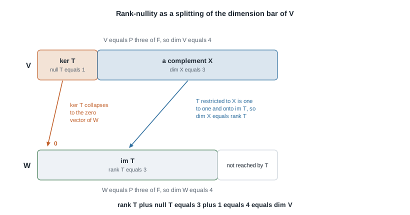
The figure is that proof, drawn. The vectors \(x_1, \dots, x_{n-k}\) span a complement \(X\) of \(\ker T\) in \(V\); the independence argument says \(T|_X\) is injective and the spanning argument says it reaches all of \(\operatorname{im} T\), so \(T|_X \colon X \to \operatorname{im} T\) is a bijection while \(\ker T\) is crushed to \(0\). The dimensions have nowhere to go but \(\dim X = \operatorname{rank} T\). Note what the picture is careful about: the complement \(X\) is not unique, as Week 1 showed, and the count does not care which one you take.

Where finite-dimensionality actually enters

The theorem says nothing about \(W\), which may be infinite-dimensional: the map \(F^2 \to F^{\mathbb{N}}\) sending \((a, b)\) to \((a, b, 0, 0, \dots)\) is injective with two-dimensional image inside an infinite-dimensional codomain, and \(2 + 0 = 2\). What it needs is that \(V\) is finite-dimensional, twice over: so that \(\ker T\) has a finite basis, and so that the basis extends to a finite basis of \(V\) without Zorn’s lemma.

Drop that and the useful consequences collapse. Let \(V = W = F^{\mathbb{N}}\) and let \(R\) be the right shift, \(R(a_1, a_2, \dots) = (0, a_1, a_2, \dots)\). It is linear with \(\ker R = \{0\}\), so \(R\) is injective and \(\operatorname{null} R = 0\); but \(\operatorname{im} R\) is the proper subspace of sequences beginning with zero, so \(R\) is not surjective. In finite dimensions with \(W = V\) this cannot happen: rank-nullity would give \(\operatorname{rank} R = \dim V\), and a subspace of \(V\) of the same finite dimension as \(V\) must equal \(V\). That last step is a finite-dimensional fact, proved in Week 2 by extending a basis, and it is exactly what fails here. The left shift \(L(a_1, a_2, \dots) = (a_2, a_3, \dots)\) makes the point from the other side: surjective, with one-dimensional kernel spanned by \((1, 0, 0, \dots)\). For an operator on a finite-dimensional space, injective, surjective and bijective coincide; on \(F^{\mathbb{N}}\), \(R\) and \(L\) pull the three apart.

Quotient spaces and the first isomorphism theorem

A count proved by choosing a basis looks contingent. The quotient construction gives a second proof that chooses nothing, and builds an object used throughout algebra.

Cosets and the well-definedness of the operations

Let \(U\) be a subspace of \(V\). For \(v \in V\) write \(v + U = \{ v + u : u \in U \}\), a subset of \(V\) called a coset of \(U\).

Lemma. \(v + U = v' + U\) if and only if \(v - v' \in U\).

Argument. If the cosets are equal then \(v = v + 0\) lies in \(v' + U\), so \(v = v' + u\) and \(v - v' = u \in U\). Conversely if \(v - v' = u_0 \in U\) then \(v + u = v' + (u_0 + u)\) for every \(u \in U\), giving \(v + U \subseteq v' + U\), and symmetry gives the other containment.

Distinct cosets are therefore disjoint: if \(w\) lies in both \(v + U\) and \(v' + U\) then \(v - w\) and \(v' - w\) lie in \(U\), hence so does \(v - v'\). The cosets partition \(V\).

Now let \(V/U\) be the set of cosets, with \[(v + U) + (v' + U) := (v + v') + U , \qquad \lambda \cdot (v + U) := (\lambda v) + U .\] This is the step students skip and the only one with content. The recipes are written using \(v\) and \(v'\), but a coset has many names and no preferred one, so the outputs must be shown independent of the name chosen. Suppose \(v + U = p + U\) and \(v' + U = p' + U\), so \(v - p \in U\) and \(v' - p' \in U\). Then \[(v + v') - (p + p') = (v - p) + (v' - p') \in U\] because \(U\) is closed under addition, so the two sums name the same coset; and \(\lambda v - \lambda p = \lambda(v - p) \in U\) because \(U\) is closed under scalar multiplication. Both checks used exactly the two closure properties of a subspace and nothing else, which is why the construction runs for subspaces and not for arbitrary subsets. The axioms are then inherited from \(V\), the zero of \(V/U\) is the coset \(0 + U = U\), and the canonical projection \(\pi(v) = v + U\) is linear by the definition of the operations, surjective by the definition of \(V/U\), and has \(\ker \pi = U\).

Proposition. If \(V\) is finite-dimensional and \(U \subseteq V\) is a subspace, then \(\dim (V/U) = \dim V - \dim U\).

Argument. Take a basis \((u_1, \dots, u_k)\) of \(U\), extend to a basis \((u_1, \dots, u_k, x_1, \dots, x_m)\) of \(V\), so \(\dim V = k + m\). Spanning: any coset is \(v + U\) with \(v = \sum_i a_i u_i + \sum_j b_j x_j\), and since \(\sum_i a_i u_i \in U\) the lemma gives \(v + U = \sum_j b_j (x_j + U)\). Independence: if \(\sum_j c_j (x_j + U) = 0 + U\) then \(\sum_j c_j x_j \in U\), so it equals \(\sum_i d_i u_i\), and independence of the full basis forces every \(c_j = 0\). Hence \(\dim(V/U) = m\).

The induced map and a second proof of the count

Theorem (first isomorphism theorem). Let \(T \colon V \to W\) be linear, with no finiteness assumed. Then \(\bar{T}(v + \ker T) = Tv\) defines an isomorphism \(\bar{T} \colon V / \ker T \to \operatorname{im} T\).

Well defined. If \(v + \ker T = v' + \ker T\) then \(v - v' \in \ker T\) by the lemma, so \(Tv - Tv' = T(v - v') = 0\) and the proposed value does not depend on the representative.

Linear. By the quotient operations and then linearity of \(T\), \[\bar{T}\big( (v + \ker T) + \lambda (v' + \ker T) \big) = T(v + \lambda v') = Tv + \lambda \, Tv' = \bar{T}(v + \ker T) + \lambda \, \bar{T}(v' + \ker T) .\]

Injective. If \(\bar{T}(v + \ker T) = 0\) then \(Tv = 0\), so \(v \in \ker T\) and \(v + \ker T\) is the zero of \(V/\ker T\); apply the kernel criterion.

Onto \(\operatorname{im} T\). Every element of \(\operatorname{im} T\) is \(Tv = \bar{T}(v + \ker T)\). \(\square\)

The first isomorphism theorem drawn as a commutative diagram from V through V mod ker T to im T inside W.

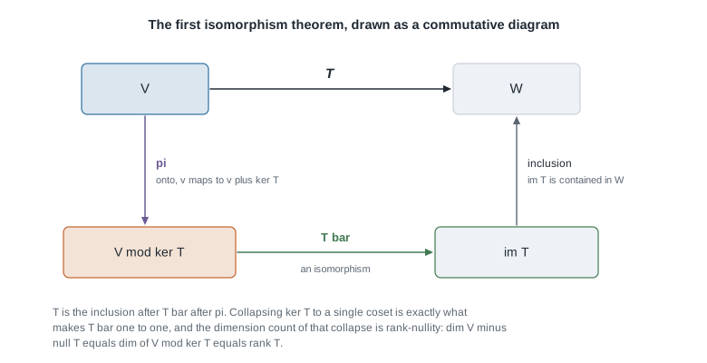
Read the diagram as a factorisation. The map \(T\) goes across the top; it also goes round the other three sides — first \(\pi\), which forgets everything but which coset a vector lies in, then the bijection \(\bar{T}\), then the inclusion into \(W\). The two routes agree, and that makes visible that \(T\) does two things in a fixed order: it collapses, then it embeds.

Now the second proof. Assume \(V\) finite-dimensional, and first note a one-line lemma: an isomorphism carries a basis to a basis. If \(\Phi \colon X \to Y\) is a linear bijection and \((z_1, \dots, z_m)\) is a basis of \(X\), then \((\Phi z_1, \dots, \Phi z_m)\) spans \(Y\) because \(\Phi\) is onto and \(\Phi(\sum a_i z_i) = \sum a_i \Phi z_i\), and is independent because \(\sum c_i \Phi z_i = 0\) gives \(\Phi(\sum c_i z_i) = 0\), hence \(\sum c_i z_i = 0\) by injectivity. So isomorphic finite-dimensional spaces have equal dimension, and applying this to \(\bar{T}\) with the quotient dimension formula, \[\operatorname{rank} T = \dim \operatorname{im} T = \dim \big( V / \ker T \big) = \dim V - \operatorname{null} T .\]

What did the second derivation buy? The first chose a basis and an extension, then verified a count. The second names the reason: \(\operatorname{im} T\) is \(V\) with \(\ker T\) collapsed, up to isomorphism, and collapsing drops dimension by exactly the dimension collapsed. Only the final equality needs finite-dimensionality; the isomorphism \(V/\ker T \cong \operatorname{im} T\) holds for every linear map between every pair of spaces over \(F\).

Worked example — differentiation on \(P_3(F)\) and the effect of the characteristic

Let \(P_3(F)\) be the formal polynomials over \(F\) of degree at most three, with ordered basis \(\mathcal{B} = (1, x, x^2, x^3)\), so \(\dim P_3(F) = 4\). Define \(D \colon P_3(F) \to P_3(F)\) on that basis by \(D(1) = 0\), \(D(x) = 1\), \(D(x^2) = 2x\), \(D(x^3) = 3x^2\) and extend linearly — a legitimate definition by the determination theorem, since naming the image of each basis vector is all that is required. So for \(p = a_0 + a_1 x + a_2 x^2 + a_3 x^3\), \[D p = a_1 + 2 a_2 \, x + 3 a_3 \, x^2 .\] “Formal” matters over a finite field: we differentiate expressions, not functions, so \(\dim P_3(\mathbb{F}_2) = 4\) even though \(x^2\) and \(x\) define the same function on \(\mathbb{F}_2\).

Working, characteristic zero. Take \(F = \mathbb{Q}\), \(\mathbb{R}\) or \(\mathbb{C}\), where no nonzero integer is zero.

1. Kernel. \(Dp = 0\) means \(a_1 = 0\), \(2a_2 = 0\), \(3a_3 = 0\) in \(F\). Since \(2 \ne 0\) and \(3 \ne 0\) and \(F\) is a field, each forces its coefficient to vanish, so \(\ker D = \operatorname{span}(1)\), the constants, and \(\operatorname{null} D = 1\).
2. Image. The image is spanned by the images of a basis, \(\operatorname{span}(0, 1, 2x, 3x^2)\). As \(2\) and \(3\) are invertible, this equals \(\operatorname{span}(1, x, x^2) = P_2(F)\), so \(\operatorname{rank} D = 3\).
3. Count. \(3 + 1 = 4 = \dim P_3(F)\), as required.

Working, characteristic three. Take \(F = \mathbb{F}_3\), where \(3 = 0\) but \(2 \ne 0\). The formula is unchanged, but its last coefficient now vanishes identically: \[Dp = a_1 + 2a_2 \, x + 0 \cdot x^2 = a_1 + 2 a_2 \, x .\]

1. Kernel. \(Dp = 0\) now means \(a_1 = 0\) and \(2a_2 = 0\); since \(2 \ne 0\) in \(\mathbb{F}_3\) the second gives \(a_2 = 0\), while \(a_0\) and \(a_3\) are unconstrained. So \(\ker D = \operatorname{span}(1, x^3)\) and \(\operatorname{null} D = 2\). Check one vector directly: \(D(x^3) = 3x^2 = 0\), so a nonconstant polynomial has entered the kernel.
2. Image. Every value lies in \(\operatorname{span}(1, x)\), and both are attained: \(1 = D(x)\), and \(x = D(2x^2)\) since \(D(2x^2) = 4x = x\) in \(\mathbb{F}_3\). So \(\operatorname{im} D = \operatorname{span}(1, x)\) and \(\operatorname{rank} D = 2\).
3. Count. \(2 + 2 = 4\). The theorem holds with different numbers on both sides.

A table comparing kernel, image, nullity and rank of differentiation in characteristic zero and three.

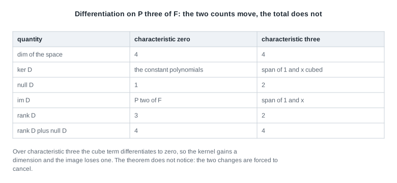
The table carries the lesson. What the theorem constrains is the total, and the total is fixed at \(\dim V = 4\) by the source space alone; the split is not fixed and moves with the field. Over \(\mathbb{F}_2\), where \(2 = 0\) and \(3 = 1\), the same computation gives \(Dp = a_1 + a_3 x^2\), so \(\ker D = \operatorname{im} D = \operatorname{span}(1, x^2)\) and \(2 + 2 = 4\) once more — with the curiosity that \(D^2 = 0\) there. What this establishes: rank-nullity is insensitive to the field, while rank and nullity separately are not. What it does not establish: that \(D\) is the same map in each case. It is a different map on a different space each time, sharing only a formula.

The same reasoning, transferred

Run the identical three steps on coordinates. Let \(F = \mathbb{R}\) and \[A = \begin{pmatrix} 1 & 2 & 0 & 1 \\ 2 & 4 & 1 & 4 \\ 1 & 2 & 1 & 3 \end{pmatrix} ,\] read as \(T \colon \mathbb{R}^4 \to \mathbb{R}^3\), \(Tx = Ax\). Subtracting twice row one from row two gives \((0, 0, 1, 2)\); subtracting row one from row three gives \((0, 0, 1, 2)\) as well, so the third row repeats the second and clears: \[\begin{pmatrix} 1 & 2 & 0 & 1 \\ 0 & 0 & 1 & 2 \\ 0 & 0 & 0 & 0 \end{pmatrix} ,\] with pivots in columns one and three. So \(\operatorname{rank} T = 2\), the free variables are \(x_2\) and \(x_4\), and \(\operatorname{null} T = 2\) with \(2 + 2 = 4\). Exhibit the kernel rather than asserting it: the equations are \(x_1 + 2x_2 + x_4 = 0\) and \(x_3 + 2x_4 = 0\), so \((x_2, x_4) = (1, 0)\) gives \((-2, 1, 0, 0)\) and \((x_2, x_4) = (0, 1)\) gives \((-1, 0, -2, 1)\). Check both against the original matrix: \(-2(1, 2, 1) + (2, 4, 2) = (0, 0, 0)\), and \(-(1, 2, 1) - 2(0, 1, 1) + (1, 4, 3) = (0, 0, 0)\). The image is spanned by the pivot columns \((1, 2, 1)\) and \((0, 1, 1)\), since column two is twice column one and column four is column one plus twice column three, as \((1, 2, 1) + (0, 2, 2) = (1, 4, 3)\). So \(\operatorname{im} T\) is the plane \(\{ y \in \mathbb{R}^3 : y_1 - y_2 + y_3 = 0 \}\), which both spanning vectors satisfy.

What stayed the same: the theorem, the three-step procedure, and the source dimension fixing the total. What changed: the space is coordinates rather than polynomials, the work is row reduction rather than reading off a formula, and this map is not surjective, since \(\operatorname{rank} T = 2 < 3\). Carry that last point into the next section.

Second worked example — building \(\mathbb{R}^3 / U\) by hand for \(U\) the \(z\)-axis

Let \(V = \mathbb{R}^3\) and \(U = \operatorname{span}(e_3) = \{ (0, 0, t) : t \in \mathbb{R} \}\), the \(z\)-axis. The construction above says \(V/U\) exists; this makes it something you can point at.

Step 1: name the cosets. By definition \(v + U = \{ (v_1, v_2, v_3 + t) : t \in \mathbb{R} \}\), the vertical line through \(v\). Two vectors share a coset exactly when their difference is vertical, that is, when their first two coordinates agree. So the cosets are the vertical lines of \(\mathbb{R}^3\), one through each vector of the \(xy\)-plane.

Cosets of the z-axis in R three drawn as parallel vertical lines through a plane.

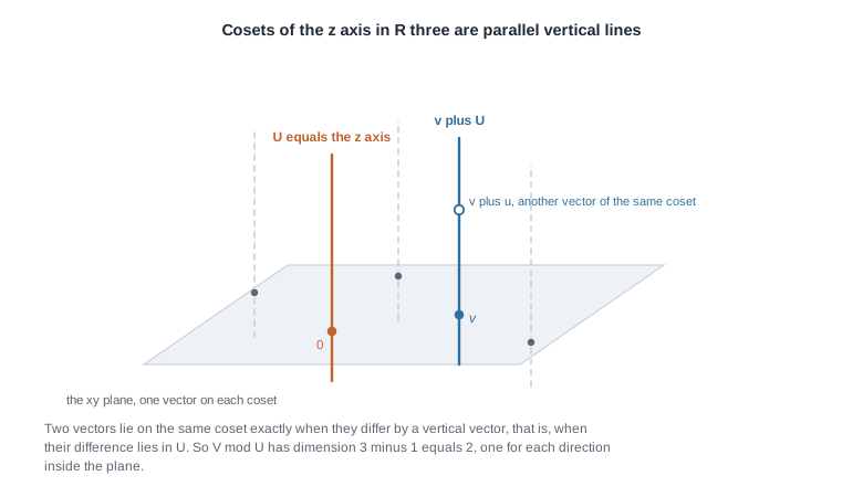
Step 2: add two cosets. Take \(v = (1, 2, 0)\) and \(v' = (3, -1, 5)\). The recipe gives \((4, 1, 5) + U\). Redo it with different names for the same two cosets: \((1, 2, 7)\) names the first, since \((1, 2, 7) - (1, 2, 0) = (0, 0, 7) \in U\), and \((3, -1, 0)\) names the second, since \((3, -1, 0) - (3, -1, 5) = (0, 0, -5) \in U\). The recipe now gives \((4, 1, 7) + U\), and the two agree because \((4, 1, 7) - (4, 1, 5) = (0, 0, 2) \in U\). That is well-definedness in front of you, and the figure shows why it had to hold: changing representative slides you along a vertical line, and vertical slides are invisible to the coset.

Step 3: scale a coset. With \(\lambda = 3\) and the coset \((1, 2, 0) + U\), the recipe gives \((3, 6, 0) + U\); with the representative \((1, 2, 7)\) it gives \((3, 6, 21) + U\), and \((3, 6, 21) - (3, 6, 0) = (0, 0, 21) \in U\).

Step 4: count and identify. The dimension proposition gives \(\dim (V/U) = 3 - 1 = 2\); taking the basis \((e_1, e_2, e_3)\) of \(\mathbb{R}^3\) with \((e_3)\) spanning \(U\), it says \((e_1 + U, e_2 + U)\) is a basis of \(V/U\). The map \(\Phi\big( (a, b, c) + U \big) = (a, b)\) is well defined by exactly the calculation of Step 2, is linear, and is a bijection, so \(V/U \cong \mathbb{R}^2\).

What this does not establish. It is tempting to conclude \(V/U\) is the \(xy\)-plane. It is not: elements of \(V/U\) are vertical lines, elements of the \(xy\)-plane are vectors. What is true is that for any complement \(X\) of \(U\), the restriction \(\pi|_X \colon X \to V/U\) is an isomorphism, since \(\ker(\pi|_X) = X \cap U = \{0\}\) and \(\dim X = 2 = \dim(V/U)\). Take \(X_1\) the \(xy\)-plane and \(X_2 = \operatorname{span}\big( (1, 0, 1), (0, 1, 0) \big)\), also a complement because \(a(1,0,1) + b(0,1,0) = (a, b, a)\) is vertical only when \(a = b = 0\). Both give isomorphisms, but they disagree about which vector represents the coset \((1, 0, 0) + U\): under \(\pi|_{X_1}\) it comes from \((1, 0, 0)\), under \(\pi|_{X_2}\) from \((1, 0, 1)\). The quotient is canonical; identifying it with a subspace of \(V\) is a choice, and Week 1’s non-uniqueness of complements is what makes the choice real.

The misreading to avoid

The sentence to dismantle: “Rank-nullity says a map from a four-dimensional space to a three-dimensional space has a one-dimensional kernel.” It says no such thing. It says \(\operatorname{null} T = 4 - \operatorname{rank} T\), and the only constraint the codomain imposes is \(\operatorname{rank} T \le \dim W = 3\), because \(\operatorname{im} T\) is a subspace of \(W\). Combining gives \(\operatorname{null} T \ge 1\) — at least one, never exactly one on this evidence. The extreme case is the zero map \(\mathbb{R}^4 \to \mathbb{R}^3\), perfectly linear, with \(\operatorname{rank} T = 0\) and \(\operatorname{null} T = 4\); the transferred example sits between the extremes at \(2\) and \(2\). The correct reading has two clauses: the theorem is an equation involving the rank, and separately \(\operatorname{rank} T \le \min(\dim V, \dim W)\). Only knowing \(T\) surjective pins the nullity down.

A second misreading is quieter and more damaging: “\(V/U\) is a subspace of \(V\).” It is not, and it is not even a subset of \(V\). An element of \(V\) is a vector; an element of \(V/U\) is a coset, that is, a subset of \(V\), and the zero of \(V/U\) is the set \(U\) rather than the vector \(0\). The two spaces are related by \(\pi\) and by the isomorphisms \(\pi|_X\) — but “related by an isomorphism” is not “equal”, and the previous example exhibited two different such isomorphisms for one \(U\). The habit worth building is to ask of any object what its elements are; for \(V/U\) they are the parallel lines in the figure, not the vectors lying on them.

One sentence on the undergraduate picture, since it is imported wholesale so often. If \(Ax_0 = b\), then the solution set of \(Ax = b\) is exactly \(x_0 + \ker A\), a coset of the kernel, which is why such a set is a translate of a subspace rather than a subspace, and why quotients are the right home for the question of how many essentially different inputs give the same output.

Practice on your own

These are for checking yourself, not for submission, and no worked responses are given; each is checkable against a statement above.

1. Let \(F\) be a field in which \(2 \ne 0\) and let \(T \colon M_2(F) \to M_2(F)\) be \(T(A) = A - A^{\mathsf{T}}\). Prove \(T\) is linear, compute \(\ker T\) and \(\operatorname{im} T\) as spans of matrices you write down, and confirm the dimensions sum to \(4\). Then say what changes over \(\mathbb{F}_2\).
2. Construct linear maps \(\mathbb{R}^4 \to \mathbb{R}^3\) of rank \(0\), \(1\) and \(3\) by naming where each standard basis vector goes and invoking the determination theorem. State each nullity, verify each count, and say which map is surjective.
3. Locate every use of finite-dimensionality in the proof of rank-nullity above and say what would go wrong without each. Then give a linear map with \(V\) finite-dimensional and \(W\) infinite-dimensional and confirm the theorem still applies.
4. Let \(V = P_3(\mathbb{R})\) and \(U = \{ p \in V : p(0) = 0 \}\). Show \(U\) is a subspace, find \(\dim U\), describe its cosets in words, and prove \(p + U \mapsto p(0)\) is a well-defined isomorphism \(V/U \to \mathbb{R}\). Which theorem above makes this immediate?
5. Prove that if \(\dim V = \dim W\) is finite then a linear \(T \colon V \to W\) is injective if and only if it is surjective. Then give two examples showing both hypotheses are needed: one where the dimensions differ, one where \(V\) is infinite-dimensional.

Where to read more

• The open lecture notes for MIT OpenCourseWare 18.700 Linear Algebra treat linear maps, kernel and image at about this level of abstraction, and are the closest free match to how this week is organised.
• MIT OpenCourseWare 18.06 Linear Algebra runs the matrix-first version of the same material, developing the four fundamental subspaces of a matrix rather than the kernel and image of a map. Read it as the contrast.
• Treil, Linear Algebra Done Wrong is an openly posted text whose treatment of linear transformations and kernels is close to this page’s, with more worked matrix computation.
• The optional Roman alignment for this week is Chapter 2, in the sections on linear transformations, on the kernel and image of a linear transformation, and on the rank plus nullity theorem; and Chapter 3, in the sections on quotient spaces and on the first isomorphism theorem. The textbook is optional for everything on this site — a borrowed or library copy suffices, and nothing here reproduces or adapts it. Availability and licence terms for all sources above are unsettled and are not asserted here.
• Course pages: the notes index, the syllabus, the schedule, and the resources page. The previous unit is Week 2 — independence, bases, and dimension, whose basis-extension results this page used four separate times.

Where this goes next

Everything here has been basis-free by design. The definition of a linear map mentions no basis; kernel, image, rank and nullity are defined without one; the quotient construction never chooses a representative that matters. Bases appeared only inside proofs, as scaffolding, and the second proof of rank-nullity showed that even there they can be removed. That is the habit this block is installing.

Week 4 does the opposite on purpose. It chooses an ordered basis \(\mathcal{B}\) of \(V\) and an ordered basis \(\mathcal{C}\) of \(W\) and builds the matrix \([T]_{\mathcal{C} \leftarrow \mathcal{B}}\), whose columns record where the basis vectors of \(V\) go — precisely the free data the determination theorem identified this week. It then asks the question that organises the rest of the course: when the bases change, which features of the matrix change and which do not? Rank survives, which is why the row-reduction count in the transferred example measured the map and not the matrix. Other features do not, and separating the two is the business of canonical forms. Return to the notes index for the block as a whole.