Week 6 — Orthogonal sets, orthonormal bases, and Gram-Schmidt
Where this week starts
Week 5 added exactly one piece of structure to a vector space and got a great deal of geometry in return: an inner product \(\langle u, v \rangle\), the norm \(\lVert v \rVert = \sqrt{\langle v, v \rangle}\) it induces, the Cauchy-Schwarz and triangle inequalities, and a definition of orthogonality. What it did not do is produce any orthogonal vectors. Every orthogonal pair on that page arrived already orthogonal, was checked, and was put away again. This week supplies them on demand, from any independent list you happen to hold.
That matters because of something Week 2 proved and then left alone. In a finite-dimensional space over \(F\), any two bases have the same number of members, and nothing in Weeks 1 through 4 preferred one basis to another. Introduce an inner product and that indifference ends. One kind of basis — an orthonormal one — makes coordinates free, makes lengths readable straight off the coefficients, and makes truncating an expansion a meaningful operation. Every other kind makes you solve a linear system and gives you nothing for free afterwards.
Fix the standing hypotheses now, because they run for the rest of the block. \(V\) is a vector space over \(F\) where \(F\) is \(\mathbb{R}\) or \(\mathbb{C}\), carrying an inner product; those are the only two fields this course develops the theory over. Positive-definiteness makes sense over any ordered field, \(\mathbb{Q}\) included, but only \(\mathbb{R}\) and \(\mathbb{C}\) are closed under the square roots that normalisation requires, and \(\mathbb{F}_2\) has no ordering in which to state \(\langle v, v \rangle > 0\) at all. Over \(\mathbb{C}\) the Week 5 convention stands without further comment: \(\langle u, v \rangle\) is linear in the first slot and conjugate-linear in the second, so \(\langle v, u \rangle = \overline{\langle u, v \rangle}\). Where a result needs \(\dim V\) finite this page says so, and it is worth noticing that two of the results below do not.
By the end of the week one reflex should be automatic. Meeting an expression \(v = a_1 v_1 + \dots + a_n v_n\), ask whether the \(v_i\) are orthonormal, because both the cost of finding the \(a_i\) and the meaning of dropping one of them turn on that. And handed an independent list, you should be able to produce an orthonormal one with the same span, prove that it works, and say what about it was forced and what was an accident of the order.
Why this matters beyond the definition
Here is a claim that sounds harmless and is false. Take \(\mathcal{B} = (b_1, b_2)\) with \(b_1 = (1, 0)\) and \(b_2 = (1, 1)\) in \(\mathbb{R}^2\) with the dot product, an ordered basis since the two are independent. Expand \(v = (0, 1)\): solving \(a_1 b_1 + a_2 b_2 = (0,1)\) gives \(a_2 = 1\) from the second coordinate and then \(a_1 = -1\), so \(v = -b_1 + b_2\). Now truncate — drop the last term and keep \(-b_1 = (-1, 0)\) as the “part of \(v\) inside \(\operatorname{span}(b_1)\)”. Its distance to \(v\) is \(\lVert (-1,-1) \rVert = \sqrt{2}\). But \(\operatorname{span}(b_1)\) is the horizontal axis, whose nearest point to \((0,1)\) is the origin, at distance \(1\). Truncating produced a vector further from \(v\) than the zero vector is.
That is not exotic; it is what happens whenever the basis is not orthogonal, and it is why least squares, Fourier series, and every numerical projection method insist on an orthogonal basis before truncating anything. All of Week 7 rests on the fact that against an orthogonal basis, and only when the discarded tail is orthogonal to the span of what remains, chopping off the tail of an expansion leaves the closest vector in the span of what remains. Orthonormality buys something else: the coefficient formula \(v = \sum_i \langle v, e_i \rangle e_i\) and the reading of length straight off the coefficients. It is not what makes truncation optimal.
What you will be able to do
- Prove that an orthogonal set of nonzero vectors in an inner product space is linearly independent, and name the hypothesis the proof actually consumes.
- Prove the expansion formula \(v = \sum_i \langle v, e_i \rangle e_i\) for an orthonormal basis, and explain why it replaces a linear solve by a list of inner products.
- Derive the Gram-Schmidt recursion and prove by induction that it is well defined, orthogonal at every stage, and span-preserving at every stage.
- Produce the \(QR\) factorisation of a matrix with independent columns and prove \(R\) is upper triangular with positive diagonal.
- Prove Bessel’s inequality for any orthonormal list, decide when it is strict, and state which extra hypothesis upgrades it to Parseval’s identity.
- Exhibit a counterexample showing the output depends on the order of the input list, and describe precisely what is determined once the order is fixed.
Terms and notation worth fixing
| Symbol or term | What it means on this page |
|---|---|
| \(\langle u, v \rangle\) | the inner product: linear in the first slot, conjugate-linear in the second |
| \(\lVert v \rVert\) | the induced norm \(\sqrt{\langle v, v \rangle}\); a unit vector has \(\lVert v \rVert = 1\) |
| orthogonal set | a set of pairwise orthogonal vectors; note this does not exclude \(0\) |
| orthonormal set | an orthogonal set of unit vectors, so \(\langle e_i, e_j \rangle = \delta_{ij}\) |
| \(\delta_{ij}\) | the Kronecker delta: \(1\) when \(i = j\), and \(0\) otherwise |
| Fourier coefficient | the scalar \(\langle v, e_i \rangle\) that an orthonormal \(e_i\) attaches to \(v\) |
| \(w_1, \dots, w_n\) | the orthogonal list Gram-Schmidt builds; \(e_1, \dots, e_n\) is it, normalised |
| \(A = QR\) | \(Q\) has orthonormal columns, \(R\) is upper triangular with positive diagonal |
| complete orthonormal set | a maximal one, meaning no nonzero vector of \(V\) is orthogonal to every member; equivalently its closed span is \(V\), and in finite dimensions the same as spanning \(V\), so an orthonormal basis |
Orthogonal sets, independence, and free coordinates
Two facts drive everything this week, and both are short. Orthogonality forces independence, so an orthogonal list is a basis of its own span as soon as its members are nonzero. And coordinates against an orthonormal basis are computed rather than solved for. Neither fact is deep, and neither is available without an inner product, which is the point.
An orthogonal set of nonzero vectors is independent
Definition. Vectors \(u\) and \(v\) in \(V\) are orthogonal when \(\langle u, v \rangle = 0\); by conjugate symmetry the relation is symmetric, since \(\langle v, u \rangle = \overline{0} = 0\). A list \((v_1, \dots, v_m)\) is an orthogonal list when \(\langle v_i, v_j \rangle = 0\) for all \(i \ne j\), and an orthonormal list when in addition \(\lVert v_i \rVert = 1\) for every \(i\), which together read \(\langle v_i, v_j \rangle = \delta_{ij}\).
Theorem. Let \(V\) be an inner product space over \(\mathbb{R}\) or \(\mathbb{C}\) and let \((v_1, \dots, v_m)\) be an orthogonal list of nonzero vectors. Then the list is linearly independent. No finite-dimensionality is assumed anywhere.
Argument. Suppose \(a_1 v_1 + \dots + a_m v_m = 0\) for scalars \(a_i \in F\). Fix an index \(j\) and pair both sides with \(v_j\), using linearity in the first slot: \[0 = \Big\langle \sum_{i=1}^{m} a_i v_i,\; v_j \Big\rangle = \sum_{i=1}^{m} a_i \langle v_i, v_j \rangle = a_j \langle v_j, v_j \rangle = a_j \lVert v_j \rVert^2 ,\] because every term with \(i \ne j\) vanishes by orthogonality. Since \(v_j \ne 0\), positive-definiteness gives \(\lVert v_j \rVert^2 > 0\), and dividing yields \(a_j = 0\). The index \(j\) was arbitrary, so every coefficient vanishes.
Three lines, and worth reading for what they use. Only linearity in the first slot appears, so the identical computation runs over \(\mathbb{C}\) with no conjugates to track. The hypothesis \(v_j \ne 0\) is not decoration: the zero vector is orthogonal to everything, so \(\{0, v\}\) is a perfectly good orthogonal set and is dependent for the silliest possible reason. And the step that carries the proof is the passage from \(\lVert v_j \rVert^2 \ne 0\) to \(a_j = 0\), which is positive-definiteness and nothing else.
Drop positive-definiteness and the theorem dies at once. Put the indefinite form \(\langle x, y \rangle_{\ast} = x_1 y_1 - x_2 y_2\) on \(\mathbb{R}^2\); it is bilinear and symmetric, satisfying every inner product axiom except positivity. Under it \(\langle (1,1), (2,2) \rangle_{\ast} = 1 \cdot 2 - 1 \cdot 2 = 0\), so \(\{(1,1), (2,2)\}\) is an orthogonal set of two nonzero vectors — and it is plainly dependent. Week 9 studies such forms deliberately; here it is the counterexample naming the load-bearing hypothesis.
Field discipline cuts here too. Over \(\mathbb{F}_2\) the standard bilinear form on \(\mathbb{F}_2^3\) has \(\langle (1,1,0), (1,1,0) \rangle = 1 + 1 + 0 = 0\) with \((1,1,0) \ne 0\), so a nonzero vector is orthogonal to itself and no orthonormal set contains it. Over \(\mathbb{Q}\) the situation is subtler: the dot product on \(\mathbb{Q}^n\) is positive definite, so orthogonal bases exist, but \(\lVert (1,1) \rVert = \sqrt{2} \notin \mathbb{Q}\), so normalising can leave the field. Orthogonal is a rational notion; orthonormal generally is not.
Corollary. If \(\dim V = n\) is finite and \((e_1, \dots, e_n)\) is an orthonormal list in \(V\), it is an orthonormal basis of \(V\). Independence comes from the theorem, since unit vectors are nonzero; and \(n\) independent vectors in an \(n\)-dimensional space form a basis by Week 2. Finite-dimensionality is used twice there, once for the counting statement and once for \(\dim V\) to be a number at all.
Coordinates against an orthonormal basis
Theorem. Let \((e_1, \dots, e_n)\) be an orthonormal basis of a finite-dimensional inner product space \(V\). Then for every \(v \in V\), \[v = \sum_{i=1}^{n} \langle v, e_i \rangle\, e_i , \qquad \text{so} \qquad [v]_{\mathcal{E}} = \begin{pmatrix} \langle v, e_1 \rangle \\ \vdots \\ \langle v, e_n \rangle \end{pmatrix}\] in the coordinate notation of Week 4, where \(\mathcal{E} = (e_1, \dots, e_n)\).
Argument. Since \(\mathcal{E}\) is a basis there are unique scalars \(a_1, \dots, a_n\) with \(v = \sum_i a_i e_i\). Pair both sides with \(e_j\) and use linearity in the first slot: \(\langle v, e_j \rangle = \sum_i a_i \langle e_i, e_j \rangle = a_j\), because \(\langle e_i, e_j \rangle = \delta_{ij}\) kills every term but one. So the coefficient that was defined by uniqueness is computed by a single inner product.
Compare the two procedures. In an arbitrary ordered basis, finding \([v]_{\mathcal{B}}\) means solving an \(n \times n\) system, cubic in \(n\). In an orthonormal basis it means \(n\) inner products, each linear in \(n\). More important than the arithmetic saving is that the coefficients no longer depend on one another: \(\langle v, e_1 \rangle\) does not know which vectors complete the basis, so enlarging or shrinking the orthonormal list never disturbs what you already computed. In a general basis it does, as the opening example showed.
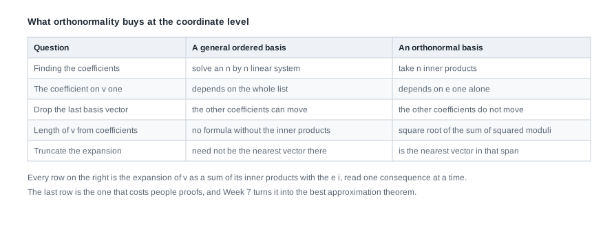
Read the table one row at a time and notice that each row is a consequence of the single expansion formula above. The last row is the one that costs people proofs, and Week 7 promotes it to a theorem. The fourth row is the identity below.
Theorem (Bessel’s inequality). Let \((e_1, \dots, e_m)\) be an orthonormal list in an inner product space \(V\) over \(\mathbb{R}\) or \(\mathbb{C}\). Neither \(V\) finite-dimensional nor the list spanning is assumed. Then for every \(v \in V\), \[\sum_{i=1}^{m} \lvert \langle v, e_i \rangle \rvert^2 \;\le\; \lVert v \rVert^2 ,\] with equality exactly when \(v \in \operatorname{span}(e_1, \dots, e_m)\).
Argument. Put \(u = \sum_{i=1}^{m} \langle v, e_i \rangle e_i\) and \(r = v - u\). For each index \(j\), expanding gives \(\langle u, e_j \rangle = \sum_i \langle v, e_i \rangle \langle e_i, e_j \rangle = \langle v, e_j \rangle\), so \(\langle r, e_j \rangle = 0\). Hence \(r\) is orthogonal to every \(e_j\) and therefore to \(u\), a combination of them. The Pythagorean identity of Week 5 gives \(\lVert v \rVert^2 = \lVert u \rVert^2 + \lVert r \rVert^2\), and expanding the first term with orthonormality, \[\lVert u \rVert^2 = \Big\langle \sum_i \langle v, e_i \rangle e_i,\; \sum_j \langle v, e_j \rangle e_j \Big\rangle = \sum_{i} \langle v, e_i \rangle \overline{\langle v, e_i \rangle} = \sum_{i} \lvert \langle v, e_i \rangle \rvert^2 ,\] the conjugate appearing because the second slot is conjugate-linear. So \(\lVert v \rVert^2 - \sum_i \lvert \langle v, e_i \rangle \rvert^2 = \lVert r \rVert^2 \ge 0\), and by positive-definiteness this is zero exactly when \(r = 0\), that is, exactly when \(v = u\) lies in the span.
Corollary (Parseval’s identity). If in addition the orthonormal list spans \(V\) — which in finite dimensions is to say it is an orthonormal basis — then equality holds for every \(v \in V\), and more generally \(\langle v, u \rangle = \sum_i \langle v, e_i \rangle \overline{\langle u, e_i \rangle}\).
The division of labour is clean: Bessel needs orthonormality alone, Parseval needs the list to span on top of it. The gap between the two sides of Bessel is exactly \(\lVert r \rVert^2\), the squared length of the part of \(v\) the list cannot see, and the second worked example computes it. One honest caveat, since Bessel carried no dimension hypothesis: for an infinite orthonormal set it still holds, and a complete orthonormal set in the maximal sense fixed in the table above is the infinite-dimensional stand-in for a basis, but recovering \(v\) from its coefficients also needs the space to be complete in its norm, and that analytic step is outside this course.
An instance in \(\mathbb{C}^2\) shows why the slot convention must be obeyed. Take \(e_1 = \tfrac{1}{\sqrt{2}}(1, i)\) and \(e_2 = \tfrac{1}{\sqrt{2}}(1, -i)\) with \(\langle u, v \rangle = u_1 \overline{v_1} + u_2 \overline{v_2}\). Then \(\langle e_1, e_1 \rangle = \tfrac{1}{2}(1 + i \cdot \overline{i}) = 1\), likewise \(\langle e_2, e_2 \rangle = 1\), and \(\langle e_1, e_2 \rangle = \tfrac{1}{2}(1 + i \cdot i) = 0\), so this is an orthonormal basis. Expand \(v = (0, 2)\): the coefficients are \(\langle v, e_1 \rangle = \tfrac{1}{\sqrt{2}}\,2\overline{i} = -i\sqrt{2}\) and \(\langle v, e_2 \rangle = \tfrac{1}{\sqrt{2}}\,2\overline{-i} = i\sqrt{2}\), and indeed \(-i\sqrt{2}\,e_1 + i\sqrt{2}\,e_2 = -i(1,i) + i(1,-i) = (-i, 1) + (i, 1) = (0,2)\). Written the other way round as \(\langle e_i, v \rangle\) you get the conjugates, which reassemble to \((0,-2)\). The formula is \(v = \sum_i \langle v, e_i \rangle e_i\), in that order, always. Parseval checks too: \(2 + 2 = 4 = \lVert (0,2) \rVert^2\).
Gram-Schmidt as a construction and a factorisation
The previous section argued that orthonormal bases are worth having. It did not produce one, and for all it said they might be rare. They are not: every finite-dimensional inner product space has one, and the proof is an algorithm you can run on paper. It takes an ordered independent list and walks along it, at each stage removing from the next vector everything already lying in the span built so far.
The recursion, and why it works
The single step is the picture the whole algorithm repeats. Given a nonzero \(w_1\) and a vector \(v_2\), we want \(w_2 = v_2 - c\,w_1\) orthogonal to \(w_1\). Impose the condition and solve for the scalar: \(0 = \langle v_2 - c w_1, w_1 \rangle = \langle v_2, w_1 \rangle - c \lVert w_1 \rVert^2\), so \[c = \frac{\langle v_2, w_1 \rangle}{\langle w_1, w_1 \rangle} ,\] legitimate precisely because \(w_1 \ne 0\) makes the denominator positive. There is exactly one such \(c\), so the step has no free parameter at all.
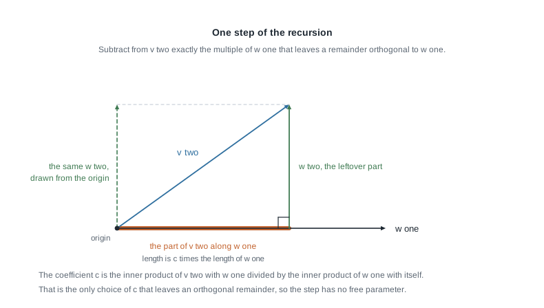
The figure shows the step as a decomposition rather than a formula: \(v_2\) splits into the part along \(w_1\), drawn on the horizontal, and the remainder, drawn where it is formed and again from the origin so you can read it as a vector in its own right. The right angle at the foot is the defining condition, and \(c\) is whatever makes that angle right.
Theorem (Gram-Schmidt). Let \(V\) be an inner product space over \(\mathbb{R}\) or \(\mathbb{C}\) and let \((v_1, \dots, v_n)\) be a linearly independent list in \(V\). Define \(w_1 = v_1\) and, for \(k = 2, \dots, n\), \[w_k = v_k - \sum_{i=1}^{k-1} \frac{\langle v_k, w_i \rangle}{\langle w_i, w_i \rangle}\, w_i .\] Then for every \(k\): (i) \(w_k\) is defined and \(w_k \ne 0\); (ii) \(\langle w_k, w_j \rangle = 0\) for all \(j < k\); and (iii) \(\operatorname{span}(w_1, \dots, w_k) = \operatorname{span}(v_1, \dots, v_k)\). Setting \(e_k = w_k / \lVert w_k \rVert\) gives an orthonormal list with the same property (iii).
Argument. Induct on \(k\). For \(k = 1\) there is nothing to subtract, \(w_1 = v_1 \ne 0\) because a member of an independent list is nonzero, and the spans agree. Suppose (i), (ii), (iii) hold below \(k\). Then \(w_1, \dots, w_{k-1}\) are nonzero, so every denominator \(\langle w_i, w_i \rangle = \lVert w_i \rVert^2\) is strictly positive and the formula for \(w_k\) makes sense.
Orthogonality: fix \(j < k\) and pair with \(w_j\), using linearity in the first slot, \[\langle w_k, w_j \rangle = \langle v_k, w_j \rangle - \sum_{i=1}^{k-1} \frac{\langle v_k, w_i \rangle}{\langle w_i, w_i \rangle} \langle w_i, w_j \rangle = \langle v_k, w_j \rangle - \frac{\langle v_k, w_j \rangle}{\langle w_j, w_j \rangle}\,\langle w_j, w_j \rangle = 0 ,\] since the inductive hypothesis kills every term of the sum except \(i = j\). No conjugate appeared, because each \(w_i\) entered the second slot only through that inductive orthogonality.
Nonvanishing: the subtracted sum is a combination of \(w_1, \dots, w_{k-1}\), hence by (iii) an element of \(\operatorname{span}(v_1, \dots, v_{k-1})\). If \(w_k\) were \(0\) we would have \(v_k \in \operatorname{span}(v_1, \dots, v_{k-1})\), contradicting independence. That is the only place independence is used, and it is used exactly there.
Spans: the same display shows \(w_k \in \operatorname{span}(v_1, \dots, v_k)\), which with the inductive hypothesis gives one inclusion. Conversely \(v_k = w_k + \sum_{i < k} c_i w_i\) for the stated \(c_i\), so \(v_k \in \operatorname{span}(w_1, \dots, w_k)\), and the inductive hypothesis places \(v_1, \dots, v_{k-1}\) there too; hence the reverse inclusion. Finally, dividing each \(w_k\) by its own positive length changes no span and no orthogonality relation.
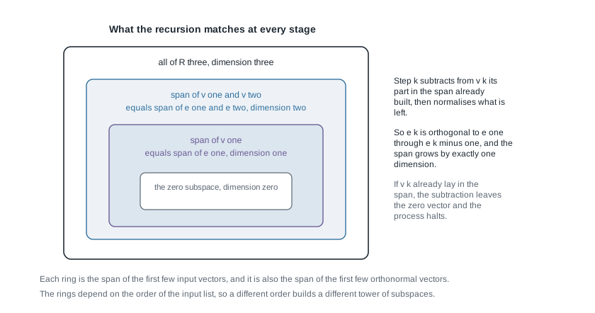
Statement (iii) is what the figure carries: at each stage the algorithm sits inside the same tower of subspaces the input list generates, adding exactly one dimension per step and never straying outside. That is stronger than merely producing an orthonormal basis of the whole span, and it is what makes \(R\) triangular below. It also makes the failure mode visible. If the input list is dependent, let \(k\) be least with \(v_k \in \operatorname{span}(v_1, \dots, v_{k-1})\); the \(k\)-th step produces \(w_k = 0\) exactly, and then both normalising \(w_k\) and running the next subtraction divide by \(\langle w_k, w_k \rangle = 0\). The process does not degrade gracefully — it halts, and where it halts names the redundant vector.
Corollary. Every finite-dimensional inner product space over \(\mathbb{R}\) or \(\mathbb{C}\) has an orthonormal basis, and every orthonormal list in such a space extends to an orthonormal basis. For the first, take any basis (Week 2 supplies one in finite dimensions) and run the theorem. For the second, note that on an already orthonormal \((v_1, \dots, v_j)\) the recursion returns the list unchanged — each subtraction removes nothing and each length is already \(1\) — so extend it to a basis by Week 2 and run Gram-Schmidt on the result.
Normalisation and the \(QR\) factorisation
Write the construction in matrix form and it becomes a factorisation you have probably met as a black box. Let \(A\) be an \(m \times n\) real matrix whose columns \(v_1, \dots, v_n\) are linearly independent, so \(n \le m\), with the standard dot product on \(\mathbb{R}^m\). Independence is a genuine hypothesis, and it is exactly what the theorem above needed.
Run Gram-Schmidt on the columns to get \(e_1, \dots, e_n\). Since \(v_k \in \operatorname{span}(v_1, \dots, v_k) = \operatorname{span}(e_1, \dots, e_k)\), the expansion theorem applied inside that subspace gives \[v_k = \sum_{i=1}^{k} \langle v_k, e_i \rangle\, e_i ,\] a sum stopping at \(i = k\) rather than running to \(n\). Let \(Q\) have columns \(e_1, \dots, e_n\) and define \(R\) by \(R_{ik} = \langle v_k, e_i \rangle\) for \(i \le k\) and \(R_{ik} = 0\) otherwise. The display says precisely that column \(k\) of \(QR\) is \(v_k\), so \(A = QR\) with \(R\) upper triangular. Two properties come free. First \(Q^{\mathsf{T}}Q = I_n\), since entry \((i,j)\) of that product is \(\langle e_i, e_j \rangle = \delta_{ij}\) — note \(I_n\), not \(I_m\); the other product \(QQ^{\mathsf{T}}\) is a different object that Week 7 identifies as the projection onto the column space. Second, writing \(v_k = w_k + (\text{a combination of } e_1, \dots, e_{k-1})\) and pairing with \(e_k\) leaves \(R_{kk} = \langle w_k, e_k \rangle = \lVert w_k \rVert > 0\), so \(R\) is triangular with no zero on the diagonal and is therefore invertible.
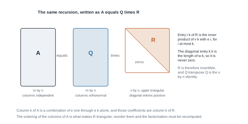
The block picture keeps the two shapes apart: \(Q\) inherits the tall shape of \(A\) while \(R\) is square of size \(n\), and the triangle records statement (iii), since column \(k\) of \(A\) involves only \(e_1\) through \(e_k\). Reorder the columns of \(A\) and the triangle is destroyed until you recompute — the same order-dependence the misreading section returns to.
Proposition (what the order determines). Let \((v_1, \dots, v_n)\) be independent, and suppose both \((e_1, \dots, e_n)\) and \((f_1, \dots, f_n)\) are orthonormal lists with \(\operatorname{span}(e_1, \dots, e_k) = \operatorname{span}(v_1, \dots, v_k) = \operatorname{span}(f_1, \dots, f_k)\) for every \(k\). Then \(f_k = c_k e_k\) with \(\lvert c_k \rvert = 1\) for each \(k\); over \(\mathbb{R}\) that means \(f_k = \pm e_k\). If moreover \(\langle v_k, e_k \rangle\) and \(\langle v_k, f_k \rangle\) are both real and positive, then \(f_k = e_k\) for every \(k\).
Argument. Fix \(k\). Since \(f_k \in \operatorname{span}(e_1, \dots, e_k)\), expansion gives \(f_k = \sum_{i \le k} \langle f_k, e_i \rangle e_i\). For \(i < k\) the hypothesis puts \(e_i \in \operatorname{span}(f_1, \dots, f_{k-1})\), and \(f_k\) is orthogonal to each of \(f_1, \dots, f_{k-1}\) hence to their span, so \(\langle f_k, e_i \rangle = 0\). Only the top term survives: \(f_k = c_k e_k\) with \(c_k = \langle f_k, e_k \rangle\), and \(1 = \lVert f_k \rVert = \lvert c_k \rvert\). Under the positivity hypothesis \(\langle v_k, f_k \rangle = \overline{c_k}\,\langle v_k, e_k \rangle\) forces \(\overline{c_k}\) to be a positive real of modulus one, so \(c_k = 1\).
Read as a statement about matrices, this is uniqueness of \(QR\): if \(A = QR = Q'R'\) with both \(Q\)’s having orthonormal columns and both \(R\)’s upper triangular with positive diagonal, then \(Q = Q'\) and \(R = R'\), since the columns satisfy the span condition and \(R_{kk} > 0\) is the positivity. Drop the sign convention and you get \(2^n\) factorisations over \(\mathbb{R}\), one per choice of signs.
Worked example — Gram-Schmidt in the standard geometry of R three
Work in \(\mathbb{R}^3\) with the dot product \(\langle x, y \rangle = x_1y_1 + x_2y_2 + x_3y_3\), and take the ordered list \[v_1 = (1,1,1), \qquad v_2 = (0,1,1), \qquad v_3 = (0,0,1) .\] These are independent: the matrix with them as columns is lower triangular with \(1\)s on the diagonal, so it is invertible. The task is an orthonormal basis with matching spans, verified, and then the \(QR\) factorisation read off.
Step 1. The first vector. \(w_1 = v_1 = (1,1,1)\), with \(\langle w_1, w_1 \rangle = 1 + 1 + 1 = 3\).
Step 2. Remove the \(w_1\) part of \(v_2\). Here \(\langle v_2, w_1 \rangle = 0 + 1 + 1 = 2\), so the coefficient is \(2/3\) and \[w_2 = (0,1,1) - \tfrac{2}{3}(1,1,1) = \big(-\tfrac{2}{3}, \tfrac{1}{3}, \tfrac{1}{3}\big) = \tfrac{1}{3}(-2, 1, 1) .\] Check the step immediately: \(\langle w_2, w_1 \rangle = \tfrac{1}{3}(-2 + 1 + 1) = 0\), and \(\langle w_2, w_2 \rangle = \tfrac{1}{9}(4 + 1 + 1) = \tfrac{2}{3}\).
Step 3. Remove both parts from \(v_3\). Now \(\langle v_3, w_1 \rangle = 1\) and \(\langle v_3, w_2 \rangle = \tfrac{1}{3}\), so the coefficients are \(\tfrac{1}{3}\) and \(\tfrac{1/3}{2/3} = \tfrac{1}{2}\), giving \[w_3 = (0,0,1) - \tfrac{1}{3}(1,1,1) - \tfrac{1}{2}\cdot\tfrac{1}{3}(-2,1,1) = (0,0,1) - \big(\tfrac{1}{3},\tfrac{1}{3},\tfrac{1}{3}\big) - \big(-\tfrac{1}{3},\tfrac{1}{6},\tfrac{1}{6}\big) = \big(0, -\tfrac{1}{2}, \tfrac{1}{2}\big) .\] Coordinate by coordinate: \(0 - \tfrac13 + \tfrac13 = 0\); \(0 - \tfrac13 - \tfrac16 = -\tfrac12\); \(1 - \tfrac13 - \tfrac16 = \tfrac12\). Its squared length is \(\tfrac14 + \tfrac14 = \tfrac12\).
Step 4. Normalise. Dividing each \(w_k\) by its length and clearing fractions, \[e_1 = \tfrac{1}{\sqrt{3}}(1,1,1), \qquad e_2 = \tfrac{1}{\sqrt{6}}(-2,1,1), \qquad e_3 = \tfrac{1}{\sqrt{2}}(0,-1,1) .\] For \(e_2\): \(\lVert w_2 \rVert = \sqrt{2/3} = \sqrt{6}/3\), and \(\tfrac{1}{3}(-2,1,1)\cdot\tfrac{3}{\sqrt{6}}\) is the displayed vector. For \(e_3\): \(\lVert w_3 \rVert = 1/\sqrt{2}\) and \(w_3 = \tfrac12(0,-1,1)\), giving the same shape.
Step 5. Verify, by computing every inner product. The three pairwise products are \((1,1,1)\cdot(-2,1,1) = -2+1+1 = 0\), \((1,1,1)\cdot(0,-1,1) = 0-1+1 = 0\), and \((-2,1,1)\cdot(0,-1,1) = 0-1+1 = 0\); each is divided by a positive number, so all three vanish. The squared lengths are \(3/3 = 1\), \(6/6 = 1\), \(2/2 = 1\). So \((e_1, e_2, e_3)\) is an orthonormal list of three vectors in a three-dimensional space, hence an orthonormal basis by the corollary above.
Step 6. Read off \(QR\). With \(A\) the matrix whose columns are \(v_1, v_2, v_3\), the entries are \(R_{ik} = \langle v_k, e_i \rangle\): \[R = \begin{pmatrix} \sqrt{3} & \tfrac{2}{\sqrt{3}} & \tfrac{1}{\sqrt{3}} \\ 0 & \tfrac{\sqrt{6}}{3} & \tfrac{1}{\sqrt{6}} \\ 0 & 0 & \tfrac{1}{\sqrt{2}} \end{pmatrix} ,\] upper triangular with positive diagonal, the diagonal being exactly \(\lVert w_1 \rVert, \lVert w_2 \rVert, \lVert w_3 \rVert\). Check column two of \(QR\): \(\tfrac{2}{\sqrt{3}}e_1 + \tfrac{\sqrt{6}}{3}e_2 = \tfrac{2}{3}(1,1,1) + \tfrac{1}{3}(-2,1,1) = (0,1,1) = v_2\). Check column three: \(\tfrac{1}{\sqrt{3}}e_1 + \tfrac{1}{\sqrt{6}}e_2 + \tfrac{1}{\sqrt{2}}e_3 = \tfrac13(1,1,1) + \tfrac16(-2,1,1) + \tfrac12(0,-1,1) = \big(0,\ \tfrac13 + \tfrac16 - \tfrac12,\ \tfrac13 + \tfrac16 + \tfrac12\big) = (0,0,1) = v_3\).
What this establishes is that the ordered list has an orthonormal companion matching its spans stage by stage, recorded by an invertible triangular matrix. What it does not establish is that \((e_1, e_2, e_3)\) is in any sense the orthonormal basis attached to these three vectors; the misreading section runs the same three in another order and gets something else. Two consistency remarks. \(\det A = 1\), since \(A\) is lower triangular with unit diagonal, and \(\det R = \sqrt{3} \cdot \tfrac{\sqrt{6}}{3} \cdot \tfrac{1}{\sqrt{2}} = \tfrac{3\sqrt{2}}{3\sqrt{2}} = 1\), so \(\det Q = 1\) too. And every entry of \(A\) is rational while no diagonal entry of \(R\) is — the earlier remark about \(\mathbb{Q}\) made concrete.
The same reasoning, transferred
Move to a function space and run the identical recursion. Let \(V = C[-1,1]\), the real continuous functions on \([-1,1]\), with \(\langle f, g \rangle = \int_{-1}^{1} f(x)g(x)\,dx\), and apply Gram-Schmidt to the independent list \(1, x, x^2\).
First \(w_1 = 1\) with \(\langle w_1, w_1 \rangle = \int_{-1}^{1} 1\,dx = 2\). Next \(\langle x, 1 \rangle = \int_{-1}^{1} x\,dx = 0\), so the subtraction removes nothing and \(w_2 = x\), with \(\langle w_2, w_2 \rangle = \int_{-1}^{1} x^2\,dx = \tfrac{2}{3}\). Finally \(\langle x^2, 1 \rangle = \tfrac{2}{3}\) and \(\langle x^2, x \rangle = \int_{-1}^{1} x^3\,dx = 0\), so \[w_3 = x^2 - \frac{2/3}{2}\cdot 1 - 0 \cdot x = x^2 - \tfrac{1}{3} .\] Its squared length is \(\int_{-1}^{1}\big(x^4 - \tfrac{2}{3}x^2 + \tfrac{1}{9}\big)dx = \tfrac{2}{5} - \tfrac{4}{9} + \tfrac{2}{9} = \tfrac{2}{5} - \tfrac{2}{9} = \tfrac{8}{45}\). Normalising, \[e_1 = \tfrac{1}{\sqrt{2}}, \qquad e_2 = \sqrt{\tfrac{3}{2}}\;x, \qquad e_3 = \sqrt{\tfrac{45}{8}}\Big(x^2 - \tfrac{1}{3}\Big) = \tfrac{\sqrt{10}}{4}\big(3x^2 - 1\big) ,\] and the last is verifiable directly: \(\tfrac{10}{16}\int_{-1}^{1}(9x^4 - 6x^2 + 1)dx = \tfrac{10}{16}\big(\tfrac{18}{5} - 4 + 2\big) = \tfrac{10}{16}\cdot\tfrac{8}{5} = 1\). These are the first three Legendre polynomials up to normalisation.
What stayed the same: the recursion verbatim, the induction proving it, the matching of spans — so \(\operatorname{span}(e_1, e_2)\) is exactly the polynomials of degree at most one — and the role of independence, which here is that a nonzero polynomial of degree at most two is not the zero function on \([-1,1]\). What changed: the inner product is an integral, so each coefficient costs a calculation; the ambient space is infinite-dimensional, and the theorem never needed otherwise; and one subtraction came out free because \(\int_{-1}^{1} x\,dx = 0\). That last is an accident of \([-1,1]\), not of the method — on \([0,1]\) we would have \(\langle x, 1 \rangle = \tfrac{1}{2} \ne 0\) and the second step would do real work.
Second worked example — coordinates two ways, and what truncation loses
Keep the orthonormal basis just built together with the orthogonal list it came from, written without denominators as \[u_1 = (1,1,1), \qquad u_2 = (-2,1,1), \qquad u_3 = (0,-1,1),\] so \(e_i = u_i / \lVert u_i \rVert\) with \(\lVert u_1 \rVert^2 = 3\), \(\lVert u_2 \rVert^2 = 6\), \(\lVert u_3 \rVert^2 = 2\). Take \(v = (1,2,3)\). We find its coordinates twice, by inner products and by elimination, and then ask what truncation does.
By inner products. Against an orthogonal basis the coefficient on \(u_i\) is \(\langle v, u_i \rangle / \langle u_i, u_i \rangle\): \[\frac{\langle v, u_1 \rangle}{3} = \frac{1 + 2 + 3}{3} = 2, \qquad \frac{\langle v, u_2 \rangle}{6} = \frac{-2 + 2 + 3}{6} = \frac{1}{2}, \qquad \frac{\langle v, u_3 \rangle}{2} = \frac{0 - 2 + 3}{2} = \frac{1}{2} .\] So \(v = 2u_1 + \tfrac12 u_2 + \tfrac12 u_3\), and reassembling confirms it: \((2,2,2) + (-1, \tfrac12, \tfrac12) + (0, -\tfrac12, \tfrac12) = (1, 2, 3)\). Three divisions, no elimination, and each coefficient obtained without reference to the other two.
By solving the system. Now do it the way Week 4 would, forgetting orthogonality. Solve \(c_1 u_1 + c_2 u_2 + c_3 u_3 = (1,2,3)\) coordinate by coordinate: \[\begin{aligned} c_1 - 2c_2 &= 1, \\ c_1 + c_2 - c_3 &= 2, \\ c_1 + c_2 + c_3 &= 3. \end{aligned}\] Subtracting the second from the third gives \(2c_3 = 1\), so \(c_3 = \tfrac12\); adding them gives \(2c_1 + 2c_2 = 5\). The first equation gives \(c_1 = 1 + 2c_2\), and substituting, \(2 + 6c_2 = 5\), so \(c_2 = \tfrac12\) and \(c_1 = 2\). Identical coefficients, at three times the work — and the work grows cubically with the dimension while the inner-product route grows quadratically.
In the normalised basis, and Bessel. Scaling, \(\langle v, e_1 \rangle = 6/\sqrt{3} = 2\sqrt{3}\), \(\langle v, e_2 \rangle = 3/\sqrt{6} = \sqrt{6}/2\), \(\langle v, e_3 \rangle = 1/\sqrt{2} = \sqrt{2}/2\). Parseval says the squares add to \(\lVert v \rVert^2\): indeed \(12 + \tfrac{6}{4} + \tfrac{2}{4} = 12 + \tfrac{3}{2} + \tfrac{1}{2} = 14 = 1 + 4 + 9\). Truncate to the first two and Bessel becomes strict: \(12 + \tfrac{3}{2} = \tfrac{27}{2} < 14\), with gap \(\tfrac{1}{2} = \lvert \langle v, e_3 \rangle \rvert^2\), exactly the squared length of the discarded piece. It is strict because \(v \notin \operatorname{span}(e_1, e_2)\), which is the equality condition of the theorem doing its job.
What truncation gives, and what it costs elsewhere. Truncating the orthonormal expansion leaves \(2u_1 + \tfrac12 u_2 = (1, \tfrac52, \tfrac52)\), with residual \(\tfrac12 u_3 = (0,-\tfrac12,\tfrac12)\), orthogonal to both \(u_1\) and \(u_2\) by construction. Week 7 proves this makes it the nearest vector of \(\operatorname{span}(u_1, u_2)\) to \(v\); the mechanism is already visible, since any other candidate differs from it by something inside the span and Pythagoras adds that difference in quadrature. Compare the original basis. Solving \(a_1 v_1 + a_2 v_2 + a_3 v_3 = (1,2,3)\) with \(v_1 = (1,1,1)\), \(v_2 = (0,1,1)\), \(v_3 = (0,0,1)\) gives \(a_1 = 1\), then \(a_2 = 1\), then \(a_3 = 1\), so \(v = v_1 + v_2 + v_3\). But the nearest vector of \(\operatorname{span}(v_1, v_2) = \operatorname{span}(u_1, u_2)\) to \(v\) is that same \((1, \tfrac52, \tfrac52)\), and expanding it in \(v_1, v_2\) gives \(1 \cdot v_1 + \tfrac32 v_2\). The coefficient on \(v_2\) moved from \(1\) to \(\tfrac32\) when the third vector was dropped. Against the orthonormal list, nothing moved at all.
The misreading to avoid
The misreading, in the words students actually use: “Gram-Schmidt turns a list into the orthonormal basis, so if two of us run it on the same three vectors we must get the same thing.” You will not, unless you also agreed on the order.
Run the algorithm on the worked example’s three vectors in the reverse order \((v_3, v_2, v_1)\). First \(w_1' = (0,0,1)\), already a unit vector, so \(e_1' = (0,0,1)\). Next \(\langle (0,1,1), (0,0,1) \rangle = 1\) and \(\langle w_1', w_1' \rangle = 1\), so \(w_2' = (0,1,1) - (0,0,1) = (0,1,0)\), another unit vector, and \(e_2' = (0,1,0)\). Finally \(\langle (1,1,1), (0,0,1) \rangle = 1\) and \(\langle (1,1,1), (0,1,0) \rangle = 1\), so \(w_3' = (1,1,1) - (0,0,1) - (0,1,0) = (1,0,0)\) and \(e_3' = (1,0,0)\). The output is the standard basis listed backwards — not one vector agrees with \(e_1 = \tfrac{1}{\sqrt3}(1,1,1)\), \(e_2 = \tfrac{1}{\sqrt6}(-2,1,1)\), \(e_3 = \tfrac{1}{\sqrt2}(0,-1,1)\), and not even the intermediate subspaces agree, since the first run built the line through \((1,1,1)\) and the second the line through \((0,0,1)\).
Now say what is determined, because “it depends on the order, so it is arbitrary” overcorrects. Fix the ordered input list. The tower \(\operatorname{span}(v_1) \subseteq \operatorname{span}(v_1, v_2) \subseteq \dots\) is then fixed, and the proposition above shows any orthonormal list matching that tower agrees with the Gram-Schmidt output up to a scalar of modulus one in each slot — a sign over \(\mathbb{R}\). Add the convention \(\langle v_k, e_k \rangle > 0\), which the algorithm satisfies automatically since \(\langle v_k, e_k \rangle = \lVert w_k \rVert\), and the output is unique. The dependence is on the ordering and nothing else.
One further dependence deserves naming, because Week 5 already warned about it. The recursion refers to \(\langle \cdot, \cdot \rangle\) at every step, so changing the inner product changes the output even with the order fixed. Put \(\langle x, y \rangle_{w'} = x_1y_1 + 2x_2y_2\) on \(\mathbb{R}^2\) and run the algorithm on \(\big((1,0),(1,1)\big)\): the first vector is already a unit vector, \(\langle (1,1),(1,0)\rangle_{w'} = 1\), so \(w_2 = (0,1)\) with \(\lVert (0,1) \rVert_{w'} = \sqrt{2}\), giving \(e_2 = (0, 1/\sqrt2)\). Under the dot product the same input gives \(e_2 = (0,1)\). Same list, same order, different geometry, different result.
A smaller misreading worth heading off: “orthogonal is basically orthonormal, so normalising is cosmetic.” Half true. For coordinates it nearly is, since an orthogonal basis of nonzero vectors gives \(v = \sum_i \frac{\langle v, u_i \rangle}{\langle u_i, u_i \rangle} u_i\) with no system to solve. But Parseval acquires weights, the diagonal of \(R\) stops being the lengths of the \(w_k\), and — the point that actually bites — over \(\mathbb{Q}\), or anywhere you insist on exact arithmetic, the orthogonal list may be available while the orthonormal one is not, because the lengths are irrational.
Practice on your own
These are for your own checking rather than for submission, and each is within reach of Weeks 1 through 6.
- Orthonormal lists of full length. Let \(\dim V = n\) be finite and let \((e_1, \dots, e_n)\) be orthonormal in \(V\). Prove it is a basis, naming both places finite-dimensionality enters. Then exhibit an orthonormal list in an infinite-dimensional inner product space that is independent, infinite, and does not span, saying which inner product you are using and on which subspace it is defined.
- Run it twice. Apply Gram-Schmidt to \((1,1,0), (1,0,1), (0,1,1)\) in \(\mathbb{R}^3\) with the dot product, carrying exact fractions and radicals, and verify all three orthonormality conditions. Then run it on the same three in the order \((0,1,1), (1,0,1), (1,1,0)\) and compare not just the outputs but the two towers of spans.
- A function-space step that is not free. In \(C[0,1]\) with \(\langle f, g \rangle = \int_0^1 fg\), apply the recursion to \(1, x, x^2\). Show that unlike the \([-1,1]\) case the second step subtracts something, obtain \(w_2\) and \(w_3\) exactly, and say what feature of \([-1,1]\) made the transferred example easier.
- A factorisation by hand. Let \(A\) be the \(3 \times 2\) matrix with columns \((1,1,0)\) and \((1,0,1)\). Compute \(Q\) and \(R\), check \(Q^{\mathsf{T}}Q = I_2\) and \(A = QR\) entry by entry, and confirm \(R\) is upper triangular with positive diagonal. Then swap the columns of \(A\) and explain why the old \(R\) is no longer triangular, without recomputing.
- Where the field stops you. On \(\mathbb{F}_2^3\) with the standard bilinear form, list every vector orthogonal to itself and conclude that no orthonormal basis exists. Then on \(\mathbb{Q}^2\) with the dot product, exhibit an orthogonal basis with rational entries and prove that no orthonormal basis of \(\mathbb{Q}^2\) contains a scalar multiple of \((1,1)\).
Where to read more
This page is self-contained, but a second treatment in a different voice is often what makes a construction settle. The three addresses below are offered online at no cost by their providers; availability and licence terms are as those providers state them, and none of that is confirmed here.
- MIT OpenCourseWare 18.700 Linear Algebra — a proof-based course whose treatment of orthonormal bases and Gram-Schmidt runs parallel to this week, with the same emphasis on the span-matching statement.
- Linear Algebra Done Wrong by Sergei Treil — an abstract-first text developing orthogonal sets, Gram-Schmidt, and the orthogonal decomposition in the order used here.
- MIT OpenCourseWare 18.06 Linear Algebra — the computational complement, useful for seeing \(QR\) exercised on explicit numerical arrays.
- The optional Roman alignment for this week is the chapter on inner product spaces, in the sections on orthogonal sets, orthonormal bases, and the Gram-Schmidt orthogonalisation process. That text is an optional reference: a borrowed or library copy suffices, purchase is never required for anything here, and nothing from it is reproduced on this page.
- Course pages: the notes overview, the syllabus, the schedule, and the resources page. The learning management system remains authoritative for section logistics and graded details.
Where this goes next
You now hold a supply of orthonormal bases, a proof that they exist in every finite-dimensional inner product space over \(\mathbb{R}\) or \(\mathbb{C}\), and the two facts that make them worth the trouble. You also know what the construction does not give — a canonical basis — and you have seen the part of \(v\) an incomplete orthonormal list cannot see, measured by the gap in Bessel’s inequality.
That gap is the subject of the next unit. Week 7, on orthogonal projections, best approximation, and least squares, takes the truncation computed above and proves it is the closest vector in the subspace, turns \(v \mapsto \sum_i \langle v, e_i \rangle e_i\) into an operator satisfying \(P^2 = P\) and \(P = P^{*}\), and derives the normal equations that fit a line to data no line passes through. Week 8 then identifies \(\operatorname{im} P\) and \(\ker P\) as a subspace and its orthogonal complement, and Week 9 asks what survives when the form is no longer positive definite. To look back: Week 5 carries the inner product axioms, Cauchy-Schwarz, and the Pythagorean identity used repeatedly here, Week 2 supplies the basis-extension results the corollaries lean on, and the notes index and course home page list everything available.