Week 9 — Bilinear forms, quadratic forms, congruence, and inertia
Where this week starts
Four weeks of geometry rested on one object. Week 5 put an inner product on a space and read a norm off it, Week 6 built orthonormal bases by Gram-Schmidt, Week 7 projected onto subspaces, and Week 8 produced \(U^{\perp}\), the adjoint \(T^{*}\), and the four fundamental subspaces. Every result there used the same three properties of \(\langle u, v \rangle\): linearity in the first slot, symmetry over \(\mathbb{R}\) or conjugate symmetry over \(\mathbb{C}\), and positive definiteness, meaning \(\langle v, v \rangle > 0\) for every \(v \ne 0\). The first two are structural and cheap. The third is expensive, and this week removes it.
What survives the removal is a bilinear form: a scalar-valued \(B(u, v)\), linear in each argument separately, with no promise that \(B(v,v)\) is positive or even nonzero for \(v \ne 0\). Lengths go, angles go, and Week 8’s splitting \(V = U \oplus U^{\perp}\) goes with them. Then something comes back. Forms have matrices, matrices move under change of basis, and the law that moves them is neither of Week 4’s two. It is a third law, \(M \mapsto P^{\mathsf{T}} M P\), called congruence, and over \(\mathbb{R}\) it admits a classification as clean as the rank normal form: three integers settle everything.
Take the loss seriously first. Week 8 proved \(V = U \oplus U^{\perp}\) for a finite-dimensional \(U\) inside an inner product space, and used positive definiteness twice: once to normalise in Gram-Schmidt, so that \(U\) has an orthonormal basis and the projection giving \(U + U^{\perp} = V\) exists, and once to force \(u \in U \cap U^{\perp}\) to satisfy \(\langle u, u \rangle = 0\) and hence vanish. Drop the hypothesis and both halves fail. On \(\mathbb{R}^2\) let \(B(x, y) = x_1y_1 - x_2y_2\), bilinear and symmetric, and let \(U = \operatorname{span}\big((1,1)\big)\). Then \(B\big((1,1),(1,1)\big) = 1 - 1 = 0\), so \(U^{\perp} = \{ y : y_1 - y_2 = 0 \}\) is \(U\) itself, \(U + U^{\perp} = U \ne \mathbb{R}^2\), and no direct sum exists. A nonzero vector orthogonal to itself is isotropic, and forbidding those is what positive definiteness was doing.
Three habits should be automatic by Friday. When a matrix appears, ask what it records — a map, an operator, or a form — because that decides which law governs it. When someone says “diagonalise”, ask under which law, since \(P^{\mathsf{T}} M P\) and \(P^{-1} M P\) are different operations. And when a real symmetric matrix appears, ask for its signature. This unit closes the syllabus’s third content block.
Why this matters beyond the definition
Here is a claim people get wrong every term. The matrix \(M = \begin{pmatrix} 1 & 2 \\ 2 & 1 \end{pmatrix}\) has both diagonal entries positive, so its quadratic form \(q(x) = x_1^2 + 4x_1x_2 + x_2^2\) must be positive too. Evaluate at \(x = (1,-1)\): \(q = 1 - 4 + 1 = -2\). The diagonal of \(M\) records \(q\) on the two standard basis vectors only, and the off-diagonal entries are what overwhelm it. Definiteness is a statement about a whole space, never about a list of entries.
The mistake is not academic. The second-derivative test classifies a critical point by the definiteness of the Hessian of second partials, which is symmetric; maximum, minimum, and saddle are signatures \((0,n,0)\), \((n,0,0)\), and anything indefinite. Statistics asks the same of a covariance matrix, where positive semidefiniteness says no linear combination of the variables has negative variance. Reading definiteness off an unearned diagonal gets both wrong the same way.
What you will be able to do
- State what a bilinear form on a space over \(F\) is, build its matrix in an ordered basis, and prove the change-of-basis law \(M \mapsto P^{\mathsf{T}} M P\).
- Distinguish equivalence, similarity, and congruence by the object each records, and name the hypothesis under which two of them coincide.
- Recover a symmetric form from its quadratic form by polarisation, name the characteristic hypothesis this needs, and exhibit its failure over \(\mathbb{F}_2\).
- Diagonalise a real symmetric form by completing the square, produce \(P\) explicitly, and verify \(P^{\mathsf{T}} M P\) by multiplying out.
- Prove Sylvester’s law of inertia and use the signature to decide congruence of real symmetric matrices.
- Exhibit a congruent pair that is not similar and a similar pair that is not congruent.
Terms and notation worth fixing
| Symbol or term | What it means on this page |
|---|---|
| \(B(u, v)\) | a bilinear form on \(V\): linear in \(u\) for fixed \(v\), and linear in \(v\) for fixed \(u\) |
| \(M = [B]_{\mathcal{B}}\) | its matrix in the ordered basis \(\mathcal{B} = (v_1, \dots, v_n)\), with entries \(M_{ij} = B(v_i, v_j)\) |
| congruence | \(N = P^{\mathsf{T}} M P\) for an invertible \(P\); an equivalence relation on \(M_n(F)\) |
| \(q(v) = B(v, v)\) | the quadratic form of \(B\), homogeneous of degree two since \(q(\lambda v) = \lambda^2 q(v)\) |
| \(\operatorname{rad} B\) | the radical \(\{ v : B(v, u) = 0 \text{ for all } u \in V \}\); \(B\) is nondegenerate when it is \(\{0\}\) |
| isotropic vector | a \(v \ne 0\) with \(q(v) = 0\); an inner product has none, a general form may have many |
| signature \((p, m, z)\) | counts of positive, negative, and zero diagonal entries in a diagonalising basis, over \(\mathbb{R}\) |
| \(H(u, v)\) | a sesquilinear form over \(\mathbb{C}\): linear in the first slot, conjugate-linear in the second |
Bilinear forms and the matrix that records them
A linear map eats one vector and returns a vector; a bilinear form eats two and returns a scalar, linearly in each slot separately rather than jointly. That is a different kind of object, and it needs its own bookkeeping — which looks reassuringly like Week 4’s and then behaves differently.
Forms, their matrices, and the congruence law
Definition. Let \(V\) be a vector space over a field \(F\). A bilinear form on \(V\) is a function \(B \colon V \times V \to F\) with \[B(u + a u', v) = B(u, v) + a\,B(u', v), \qquad B(u, v + a v') = B(u, v) + a\,B(u, v')\] for all \(u, u', v, v' \in V\) and \(a \in F\).
Three examples at once. The dot product \(B(x,y) = x_1y_1 + \dots + x_ny_n\) on \(F^n\) works over any field, and over \(\mathbb{F}_2\) we get \(B\big((1,1),(1,1)\big) = 1 + 1 = 0\), so it is no inner product there. The form \(B(x,y) = x_1y_2 - x_2y_1\) on \(F^2\) satisfies \(B(v,v) = 0\) for every \(v\). And \(B(f,g) = \int_0^1 fg\) on \(C[0,1]\) is the Week 5 inner product, so inner products are bilinear forms and not conversely.
Definition and lemma. Let \(\dim V = n\) be finite with ordered basis \(\mathcal{B} = (v_1, \dots, v_n)\). The matrix of \(B\) relative to \(\mathcal{B}\) is \(M = [B]_{\mathcal{B}}\) with \(M_{ij} = B(v_i, v_j)\), and then \(B(u, v) = [u]_{\mathcal{B}}^{\mathsf{T}} M [v]_{\mathcal{B}}\) for all \(u, v \in V\).
Argument. Write \(u = \sum_i a_i v_i\) and \(v = \sum_j b_j v_j\), so \(a = [u]_{\mathcal{B}}\) and \(b = [v]_{\mathcal{B}}\). Expanding the first slot and then each term’s second slot, \[B(u, v) = \sum_{i=1}^{n} a_i B(v_i, v) = \sum_{i=1}^{n}\sum_{j=1}^{n} a_i b_j B(v_i, v_j) = a^{\mathsf{T}} M b .\] Conversely each \(M \in M_n(F)\) defines a form this way, and evaluating \(a^{\mathsf{T}}Mb\) at standard coordinate columns returns \(M_{ij}\), so the two constructions invert one another and no matrix is missed.
Fixed basis, and Week 4 taught you to ask what happens otherwise. Let \(\mathcal{C} = (w_1, \dots, w_n)\) be a second ordered basis and \(P = P_{\mathcal{B} \leftarrow \mathcal{C}}\) the change-of-basis matrix whose \(j\)-th column is \([w_j]_{\mathcal{B}}\), so \([v]_{\mathcal{B}} = P [v]_{\mathcal{C}}\).
Theorem (the congruence law). For \(V\) finite-dimensional over \(F\) with \(M = [B]_{\mathcal{B}}\), the matrix of the same form in \(\mathcal{C}\) is \([B]_{\mathcal{C}} = P^{\mathsf{T}} M P\), with \(P = P_{\mathcal{B} \leftarrow \mathcal{C}}\) invertible.
Argument. Substitute the coordinate identity into the lemma: \[B(u, v) = [u]_{\mathcal{B}}^{\mathsf{T}} M [v]_{\mathcal{B}} = \big(P[u]_{\mathcal{C}}\big)^{\mathsf{T}} M \big(P[v]_{\mathcal{C}}\big) = [u]_{\mathcal{C}}^{\mathsf{T}}\big(P^{\mathsf{T}} M P\big)[v]_{\mathcal{C}} .\] The matrix representing \(B\) in a given basis is unique, because evaluating at the standard coordinate columns recovers its entries one at a time; so the bracket is \([B]_{\mathcal{C}}\). Invertibility of \(P\) is Week 4’s fact that \(P_{\mathcal{C} \leftarrow \mathcal{B}}\) inverts it.
Definition. \(M, N \in M_n(F)\) are congruent when \(N = P^{\mathsf{T}} M P\) for some invertible \(P\). This is an equivalence relation: \(P = I\) gives reflexivity, \(M = (P^{-1})^{\mathsf{T}} N P^{-1}\) symmetry, and \((PQ)^{\mathsf{T}} M (PQ) = Q^{\mathsf{T}}(P^{\mathsf{T}}MP)Q\) transitivity.
Two invariants fall straight out. Congruence preserves rank, since \(P\) and \(P^{\mathsf{T}}\) are invertible and Week 4 showed invertible factors on either side leave rank alone; so \(\operatorname{rank} B\) is well defined. And it preserves symmetry, since \((P^{\mathsf{T}}MP)^{\mathsf{T}} = P^{\mathsf{T}}M^{\mathsf{T}}P\). Determinants move, but only by squares: \(\det(P^{\mathsf{T}}MP) = (\det P)^2 \det M\), so over \(\mathbb{R}\) a nonzero determinant keeps its sign.
The coordinate-free version of rank deficiency is the radical, \(\operatorname{rad} B = \{ v : B(v,u) = 0 \text{ for all } u \}\), a subspace because those conditions are linear in \(v\). In coordinates it says \([v]_{\mathcal{B}}^{\mathsf{T}} M = 0\), so the coordinate isomorphism carries it onto the null space of \(M^{\mathsf{T}}\) and rank-nullity from Week 3 gives \(\dim \operatorname{rad} B = n - \operatorname{rank} M\). Call \(B\) nondegenerate when the radical is \(\{0\}\), equivalently when \(M\) is invertible in one and hence in every basis.
Symmetry, quadratic forms, and polarisation
Definition. \(B\) is symmetric when \(B(u,v) = B(v,u)\) always, and alternating when \(B(v,v) = 0\) always. The first holds exactly when \(M^{\mathsf{T}} = M\) in one basis, hence in every basis by the congruence law.
Alternating implies skew-symmetric over any field: expanding \(0 = B(u+v, u+v)\) gives \(B(u,v) + B(v,u) = 0\). The converse needs \(2 \ne 0\) in \(F\), since skew-symmetry only yields \(2B(v,v) = 0\). This is the crack that opened in Week 1, where the symmetric-plus-skew splitting of \(M_2(F)\) collapsed over \(\mathbb{F}_2\), and it opens here for the same reason.
Definition. The quadratic form of \(B\) is \(q(v) = B(v,v)\). In coordinates \(q(x) = x^{\mathsf{T}}Mx = \sum_i M_{ii}x_i^2 + \sum_{i \ne j} M_{ij}x_ix_j\), homogeneous of degree two.
Different forms can share a quadratic form, since \(B\) and the form \(B'(u,v) = B(v,u)\) agree on the diagonal, so the real question is whether a symmetric \(B\) is recoverable from \(q\). It is, with a hypothesis.
Theorem (polarisation). Let \(F\) have characteristic not two and let \(B\) be a symmetric bilinear form on a space \(V\) over \(F\), with \(q(v) = B(v,v)\). Then \(B(u,v) = \tfrac{1}{2}\big(q(u+v) - q(u) - q(v)\big)\) for all \(u, v\), so \(q\) determines \(B\).
Argument. Bilinearity gives \(q(u+v) = B(u,u) + B(u,v) + B(v,u) + B(v,v)\), symmetry merges the middle terms into \(2B(u,v)\), and dividing by the invertible scalar \(2\) rearranges.
The failure is short and permanent. Over \(\mathbb{F}_2\) take \(V = \mathbb{F}_2^2\) and \[M_1 = \begin{pmatrix} 1 & 0 \\ 0 & 1 \end{pmatrix}, \qquad M_2 = \begin{pmatrix} 1 & 1 \\ 1 & 1 \end{pmatrix} .\] The forms differ, since \(B_1(e_1,e_2) = 0\) and \(B_2(e_1,e_2) = 1\). The quadratic forms do not: \(q_2(x) = x_1^2 + 2x_1x_2 + x_2^2 = x_1^2 + x_2^2 = q_1(x)\), because \(2 = 0\) kills the cross term. So in characteristic two the passage from \(B\) to \(q\) destroys information no formula restores, and that theory is built on a different definition. Everything below assumes characteristic not two, and mostly assumes \(F = \mathbb{R}\).
Three transformation laws, side by side
You now hold three relations on matrices, from three different questions, and confusing them is the standard way to go wrong this month. A matrix recording a map \(T \colon V \to W\) has two bases available and moves by \(A \mapsto QAP^{-1}\), equivalence, complete invariant rank. A matrix recording an operator has one basis at both ends and moves by \(A \mapsto P^{-1}AP\), similarity, whose classification takes until Week 15. A matrix recording a bilinear form has one basis in both slots and moves by \(M \mapsto P^{\mathsf{T}}MP\).
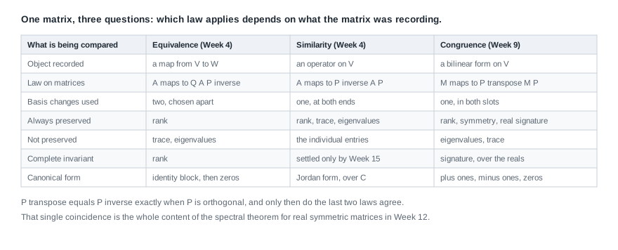
Read the table by rows and the pattern is plain. Similarity and congruence look alike on the page and are unrelated as relations, because \(P^{-1}\) and \(P^{\mathsf{T}}\) are different matrices. They agree exactly when \(P^{\mathsf{T}} = P^{-1}\), which is what orthogonal means. That single condition is the bridge between the two halves of the course: Week 12’s spectral theorem says an orthogonal \(P\) suffices to diagonalise a real symmetric matrix, and only there do the congruence data and the eigenvalues coincide.
Over \(\mathbb{C}\) the inner product was sesquilinear, and the bookkeeping runs with a conjugate inserted. A sesquilinear form \(H\) is linear in the first slot and conjugate-linear in the second, following Week 5. With \(M_{ij} = H(v_i, v_j)\) the same expansion gives \(H(u,v) = [u]_{\mathcal{B}}^{\mathsf{T}} M \overline{[v]_{\mathcal{B}}}\), and \(H\) is Hermitian, meaning \(H(v,u) = \overline{H(u,v)}\), exactly when \(M^{*} = M\) for the conjugate transpose of Week 8. A scalar equals its own transpose, so the identity also reads \(H(u,v) = [v]_{\mathcal{B}}^{*} M^{\mathsf{T}} [u]_{\mathcal{B}}\), in which the recorded matrix obeys \(K \mapsto P^{*}KP\) — conjugate congruence. Since \(H(v,v)\) is then real, definiteness and signature make sense over \(\mathbb{C}\), and every result below transfers with \(P^{\mathsf{T}}\) replaced by \(P^{*}\).
Diagonalising a symmetric form, and what the diagonal remembers
A diagonal matrix means a basis with \(B(v_i, v_j) = 0\) for \(i \ne j\) — an orthogonal basis for the form, in Week 6’s sense, but with no normalisation available. Two questions follow: does such a basis always exist, and what about the resulting diagonal is forced rather than chosen?
Every symmetric form has a diagonalising basis
Theorem. Let \(F\) have characteristic not two, let \(V\) be finite-dimensional over \(F\), and let \(B\) be a symmetric bilinear form on \(V\). Then \(V\) has an ordered basis in which the matrix of \(B\) is diagonal; equivalently, every symmetric \(M \in M_n(F)\) is congruent to a diagonal matrix.
Argument. Induct on \(n = \dim V\), the cases \(n = 0\) and \(n = 1\) being empty. Let \(n \ge 2\). If \(q(v) = 0\) for every \(v\), polarisation — legal because the characteristic is not two — gives \(B = 0\), diagonal in any basis. Otherwise pick \(u_1\) with \(c = B(u_1,u_1) \ne 0\) and let \(\varphi(v) = B(u_1, v)\), a linear functional with \(\varphi(u_1) = c \ne 0\), hence surjective onto \(F\). Rank-nullity from Week 3 makes \(X = \ker \varphi\) of dimension \(n - 1\), and \(u_1 \notin X\) forces \(\operatorname{span}(u_1) \cap X = \{0\}\), so the Week 2 dimension formula gives \(V = \operatorname{span}(u_1) \oplus X\). The restriction of \(B\) to \(X\) is symmetric and bilinear, so induction supplies a basis \((u_2, \dots, u_n)\) of \(X\) diagonalising it. In \((u_1, \dots, u_n)\) we have \(B(u_1, u_j) = \varphi(u_j) = 0\) for \(j \ge 2\) by construction and \(B(u_i,u_j) = 0\) for \(2 \le i \ne j\) by induction, so the matrix is diagonal with \(c\) upper left.
Two remarks make the proof usable. It is Gram-Schmidt with normalisation stripped out and one extra case: when the form is positive definite every nonzero \(u_1\) has \(B(u_1,u_1) \ne 0\) and you may divide by \(\sqrt{B(u_1,u_1)}\), which is exactly how Week 6 reached \(I_n\). And no determinant and no eigenvalue appeared, so the theorem holds verbatim over \(\mathbb{Q}\) or \(\mathbb{F}_5\), where eigenvalues may fail to exist. Finite-dimensionality is used, in the induction; algebraic closure is not.
The algorithm inside the proof is Lagrange’s method of completing squares, and it is what you run. Given \(q(x) = x^{\mathsf{T}}Mx\): if some \(M_{ii} \ne 0\), collect every term containing \(x_i\), complete the square to get \(M_{ii}(x_i + \ell)^2\) for a linear \(\ell\) in the other variables, and recurse on the remainder, which no longer involves \(x_i\). If every diagonal entry vanishes but some \(M_{ij} \ne 0\) with \(i \ne j\), substitute \(x_i = y_i + y_j\) and \(x_j = y_i - y_j\); the cross term becomes \(2M_{ij}(y_i^2 - y_j^2)\), nonzero on the diagonal because the characteristic is not two, and the first case applies.
Sylvester’s law of inertia
Over \(\mathbb{R}\) the diagonal entries are not themselves invariant — scaling \(u_i\) by \(t\) scales \(B(u_i,u_i)\) by \(t^2\) — but their signs are, and that is the theorem.
Theorem (Sylvester’s law of inertia). Let \(V\) be a finite-dimensional real vector space and \(B\) a symmetric bilinear form on \(V\). If one ordered basis diagonalises \(B\) with \(p\) positive, \(m\) negative and \(z\) zero diagonal entries, and another does so with \(p'\), \(m'\), \(z'\), then \(p = p'\), \(m = m'\) and \(z = z'\).
Argument. Write \(n = \dim V\). Each triple sums to \(n\), and \(p + m\) is the rank of a diagonal matrix representing \(B\), which is congruence-invariant; so \(z = z'\) and it suffices to prove \(p = p'\). Suppose \(p > p'\). Order the first basis \((u_1, \dots, u_n)\) with its positive entries first, and the second \((w_1, \dots, w_n)\) likewise. Put \(X = \operatorname{span}(u_1, \dots, u_p)\) and \(Y = \operatorname{span}(w_{p'+1}, \dots, w_n)\). For nonzero \(x = \sum_{i \le p} a_iu_i\) the cross terms vanish and \(q(x) = \sum_{i \le p} a_i^2 B(u_i,u_i) > 0\), since some \(a_i \ne 0\). For any \(y = \sum_{j > p'} b_jw_j\) the same expansion gives \(q(y) = \sum_{j > p'} b_j^2 B(w_j,w_j) \le 0\), since every entry indexed beyond \(p'\) is negative or zero. Now count. Since \(\dim X + \dim Y = p + (n - p') > n\), the Week 2 dimension formula forces \[\dim(X \cap Y) = \dim X + \dim Y - \dim(X + Y) \ge p + (n - p') - n = p - p' \ge 1 .\] Choose \(v \ne 0\) in \(X \cap Y\): then \(q(v) > 0\) and \(q(v) \le 0\), which is impossible. So \(p \le p'\), and exchanging the two bases gives \(p' \le p\).
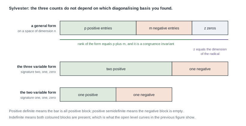
The bar is the theorem in one picture: its length is \(\dim V\), its three coloured blocks are what a diagonalising basis produces, and Sylvester says the three widths never move. Rank is the first two blocks together, the third is the radical, and the form is nondegenerate exactly when the third is empty. The two bars beneath are the forms computed later on this page, drawn to a common unit width so that their lengths are their dimensions: the three-variable form of signature \((2,1,0)\), and beneath it the shorter two-variable form of signature \((1,1,0)\).
Call \((p, m, z)\) the signature. Some texts use the single integer \(p - m\) instead; the triple carries more when \(z > 0\), so it is what this course means. Normalising finishes the classification: scaling \(u_i\) by \(1/\sqrt{|B(u_i,u_i)|}\) wherever that entry is nonzero turns the diagonal into \(p\) ones, then \(m\) entries \(-1\), then \(z\) zeros. So every real symmetric \(M\) is congruent to exactly one matrix of that shape, and two real symmetric matrices of the same size are congruent if and only if their signatures agree.
The dependence on \(\mathbb{R}\) deserves naming. Normalisation used that positive reals have real square roots, and inertia used that squares are non-negative. Over \(\mathbb{C}\) every scalar has a square root, so the \(-1\) entries scale to \(1\) and a symmetric complex matrix is congruent to \(\operatorname{diag}(I_r, 0)\) with \(r = \operatorname{rank} M\): rank alone classifies, and inertia says nothing. The same holds over any algebraically closed field of characteristic not two. Over \(\mathbb{Q}\) the classification is finer than over \(\mathbb{R}\), since \(x^2\) and \(2x^2\) share a real signature while no rational \(P\) satisfies \(P^2 \cdot 1 = 2\).
Definiteness, and the minor test we are quoting
Definition. A real symmetric form \(B\), with \(q(v) = B(v,v)\), is positive definite when \(q(v) > 0\) for all \(v \ne 0\); positive semidefinite when \(q(v) \ge 0\) for all \(v\); negative definite and negative semidefinite with the inequalities reversed; and indefinite when \(q\) takes both a positive and a negative value.
In signature terms with \(n = \dim V\): positive definite is \((n,0,0)\), positive semidefinite is \(m = 0\), negative definite is \((0,n,0)\), indefinite is \(p \ge 1\) and \(m \ge 1\). One line proves it in a diagonalising basis, where \(q(\sum a_iu_i) = \sum d_ia_i^2\) for diagonal entries \(d_i\): if every \(d_i > 0\) the sum is positive unless all \(a_i\) vanish, and if some \(d_i \le 0\) then \(q(u_i) = d_i \le 0\) at the nonzero \(u_i\). So a real inner product is precisely a positive definite symmetric bilinear form, and Weeks 5 through 8 studied one signature class out of many.
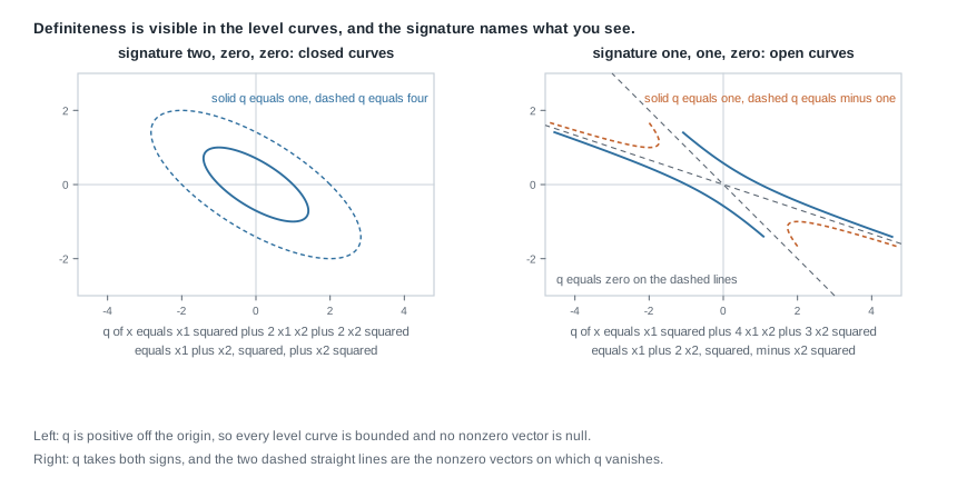
The panels make the two signatures visible. On the left is \(q(x) = x_1^2 + 2x_1x_2 + 2x_2^2 = (x_1+x_2)^2 + x_2^2\), whose level curves are bounded ovals nested about the origin because \(q\) grows in every direction; no isotropic vector exists and no straight line appears. On the right is \(q(x) = x_1^2 + 4x_1x_2 + 3x_2^2 = (x_1+2x_2)^2 - x_2^2\), whose level curves are hyperbolas opening two ways according to the sign of the level, separated by the dashed lines \(x_1 = -x_2\) and \(x_1 = -3x_2\) on which \(q\) vanishes. Those lines are the isotropic directions, and they are exactly what the definite picture lacks.
Finally the computational test, which this course quotes rather than proves because it belongs to determinant theory. Write \(\Delta_k\) for the leading principal minor of order \(k\), the determinant of the top-left \(k \times k\) submatrix. Quoted: a real symmetric \(M\) is positive definite if and only if \(\Delta_k > 0\) for every \(k = 1, \dots, n\). Also quoted: when no \(\Delta_k\) vanishes, \(m\) equals the number of sign changes in the list \(1, \Delta_1, \dots, \Delta_n\), which gives a free check on any hand computation.
Store one warning beside the test: it does not extend to semidefiniteness by relaxing the inequality. For \(M = \operatorname{diag}(0,-1)\) both leading minors are zero, hence non-negative, yet \(q(0,1) = -1 < 0\) and the form is negative semidefinite. The correct criterion needs all principal minors — every submatrix obtained by deleting the same rows and columns — to be non-negative, not merely the leading ones.
Worked example — a three-variable form diagonalised by completing the square
Work over \(\mathbb{R}\) with \(V = \mathbb{R}^3\) in the standard ordered basis, and take the symmetric form \(B\) with matrix \[M = \begin{pmatrix} 1 & 2 & 1 \\ 2 & 3 & 1 \\ 1 & 1 & 2 \end{pmatrix}, \qquad q(x) = x_1^2 + 3x_2^2 + 2x_3^2 + 4x_1x_2 + 2x_1x_3 + 2x_2x_3 ,\] reading the coefficient of \(x_i^2\) as \(M_{ii}\) and that of \(x_ix_j\) as \(M_{ij} + M_{ji} = 2M_{ij}\). Produce a diagonalising basis, exhibit the congruence matrix, verify it by multiplication, and read the signature.
Step 1. Clear \(x_1\). Its square has nonzero coefficient, so collect and complete: \[x_1^2 + 4x_1x_2 + 2x_1x_3 = (x_1 + 2x_2 + x_3)^2 - (2x_2 + x_3)^2 = (x_1+2x_2+x_3)^2 - 4x_2^2 - 4x_2x_3 - x_3^2 .\]
Step 2. Recurse. Adding back the terms free of \(x_1\) leaves \(3x_2^2 + 2x_3^2 + 2x_2x_3 - 4x_2^2 - 4x_2x_3 - x_3^2 = -x_2^2 - 2x_2x_3 + x_3^2\). Complete the square in \(x_2\), minding the negative coefficient: \(-x_2^2 - 2x_2x_3 = -\big((x_2+x_3)^2 - x_3^2\big)\), so the remainder is \(-(x_2+x_3)^2 + 2x_3^2\) and altogether \[q(x) = (x_1 + 2x_2 + x_3)^2 - (x_2 + x_3)^2 + 2x_3^2 .\]
Step 3. Name the new coordinates. Set \(y_1 = x_1 + 2x_2 + x_3\), \(y_2 = x_2 + x_3\), \(y_3 = x_3\), that is \(y = Cx\) with \[C = \begin{pmatrix} 1 & 2 & 1 \\ 0 & 1 & 1 \\ 0 & 0 & 1 \end{pmatrix}, \qquad q = y^{\mathsf{T}} D y, \qquad D = \operatorname{diag}(1,-1,2) .\] \(C\) is upper triangular with unit diagonal, hence invertible, and \(x = C^{-1}y\) makes \(P = C^{-1}\) the congruence matrix. Solving \(CP = I\) column by column, \[P = \begin{pmatrix} 1 & -2 & 1 \\ 0 & 1 & -1 \\ 0 & 0 & 1 \end{pmatrix} .\] Check it: row \((1,2,1)\) of \(C\) against the columns \((1,0,0)\), \((-2,1,0)\), \((1,-1,1)\) of \(P\) gives \(1\), then \(-2+2 = 0\), then \(1-2+1 = 0\); row \((0,1,1)\) gives \(0\), \(1\), \(-1+1 = 0\); row \((0,0,1)\) gives \(0\), \(0\), \(1\).
Step 4. Verify \(P^{\mathsf{T}} M P = D\). First \(MP\), column by column. Column one of \(P\) selects column one of \(M\), namely \((1,2,1)^{\mathsf{T}}\). Column two \((-2,1,0)^{\mathsf{T}}\) gives \(\big(-2+2,\; -4+3,\; -2+1\big) = (0,-1,-1)\). Column three \((1,-1,1)^{\mathsf{T}}\) gives \(\big(1-2+1,\; 2-3+1,\; 1-1+2\big) = (0,0,2)\). So \[MP = \begin{pmatrix} 1 & 0 & 0 \\ 2 & -1 & 0 \\ 1 & -1 & 2 \end{pmatrix} .\] Multiply on the left by \(P^{\mathsf{T}}\), whose rows are \((1,0,0)\), \((-2,1,0)\), \((1,-1,1)\). Row one selects row one of \(MP\), giving \((1,0,0)\). Row two gives \(-2(1,0,0) + (2,-1,0) = (0,-1,0)\). Row three gives \((1,0,0) - (2,-1,0) + (1,-1,2) = (0,0,2)\). Hence \(P^{\mathsf{T}}MP = D\), as claimed. The diagonalising basis is the columns of \(P\): \(u_1 = (1,0,0)\), \(u_2 = (-2,1,0)\), \(u_3 = (1,-1,1)\). Directly, \(B(u_1,u_2) = (1,0,0)\cdot(0,-1,-1) = 0\) and \(B(u_2,u_3) = (-2,1,0)\cdot(0,0,2) = 0\), using the columns of \(MP\) above.
Step 5. Read the signature, and check it twice. The diagonal \((1,-1,2)\) has two positive entries, one negative, none zero, so \((p,m,z) = (2,1,0)\): nondegenerate and indefinite. Determinants agree, since \(\det M = 1(6-1) - 2(4-1) + 1(2-3) = 5 - 6 - 1 = -2\) and \(\det D = -2\), as they must because \(\det P = 1\). Leading minors give \(\Delta_1 = 1\), \(\Delta_2 = 3 - 4 = -1\), \(\Delta_3 = -2\), so the list \(1, 1, -1, -2\) has exactly one sign change, matching \(m = 1\).
So \(M\) is congruent to \(\operatorname{diag}(1,-1,2)\) and, after scaling \(u_3\) by \(1/\sqrt{2}\), to \(\operatorname{diag}(1,-1,1)\); reordering the basis as \(u_1, u_3, u_2\) puts this in the normal form \(\operatorname{diag}(1,1,-1)\), the unique normalised representative of its class. What this does not establish is anything about eigenvalues: \(\operatorname{tr} M = 6\) while \(\operatorname{tr} D = 2\), so \(M\) and \(D\) are not similar even though they record one form.
The same reasoning, transferred
Run the identical procedure in two variables, where a picture is available. Take \(M' = \begin{pmatrix} 1 & 2 \\ 2 & 3 \end{pmatrix}\), the leading block of \(M\), with \(q'(x) = x_1^2 + 4x_1x_2 + 3x_2^2\). Completing the square gives \(q'(x) = (x_1+2x_2)^2 - 4x_2^2 + 3x_2^2 = (x_1+2x_2)^2 - x_2^2\), so \(y_1 = x_1 + 2x_2\), \(y_2 = x_2\), and \[C' = \begin{pmatrix} 1 & 2 \\ 0 & 1 \end{pmatrix}, \qquad P' = (C')^{-1} = \begin{pmatrix} 1 & -2 \\ 0 & 1 \end{pmatrix} .\] Verify: \(M'P'\) has columns \((1,2)^{\mathsf{T}}\) and \(M'(-2,1)^{\mathsf{T}} = (-2+2,\, -4+3) = (0,-1)^{\mathsf{T}}\); then \((P')^{\mathsf{T}}\) has rows \((1,0)\) and \((-2,1)\), giving \((1,0)\) and \(-2(1,0) + (2,-1) = (0,-1)\). So \((P')^{\mathsf{T}}M'P' = \operatorname{diag}(1,-1)\) and the signature is \((1,1,0)\).
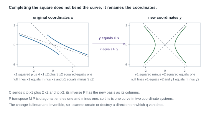
The figure shows what the algebra did. The level set \(q'(x) = 1\) is a hyperbola whose asymptotes are the isotropic lines \(x_1 = -x_2\) and \(x_1 = -3x_2\); check \(q'(1,-1) = 1 - 4 + 3 = 0\) and \(q'(3,-1) = 9 - 12 + 3 = 0\). In the new coordinates it is \(y_1^2 - y_2^2 = 1\) with asymptotes \(y_1 = \pm y_2\). The change of coordinates is linear and invertible, so it sends lines to lines and fixes the origin, and it cannot turn a curve with two isotropic directions into one with none. That is Sylvester’s law seen as geometry.
What stayed the same: the order of operations, the identification of \(P\) as the inverse of the substitution matrix, the verification by explicit multiplication, and the reading of the signature off the diagonal. What changed: the dimension dropped, one square disappeared, and the signature went from \((2,1,0)\) to \((1,1,0)\) — still indefinite, so still a hyperbola. One contrast to carry into Week 12: the eigenvalues of \(M'\) satisfy \(t^2 - 4t - 1 = 0\), so \(\lambda = 2 \pm \sqrt{5}\), one positive and one negative. Ugly numbers the congruence never computed — yet their signs match the signature, and that is no accident.
Second worked example — congruent and not similar, similar and not congruent
The point here is that the two relations cross rather than nest. Both halves use \(2 \times 2\) real matrices and integer arithmetic.
Half one: congruent, not similar. Let \(M_1 = I_2\) and \(P = \begin{pmatrix} 1 & 1 \\ 0 & 1 \end{pmatrix}\), invertible with determinant one. Then \[M_2 = P^{\mathsf{T}} M_1 P = P^{\mathsf{T}}P = \begin{pmatrix} 1 & 0 \\ 1 & 1 \end{pmatrix}\begin{pmatrix} 1 & 1 \\ 0 & 1 \end{pmatrix} = \begin{pmatrix} 1 & 1 \\ 1 & 2 \end{pmatrix} ,\] entry by entry: \(1\), \(1\), \(1\), and \(1 + 1 = 2\). So the two are congruent by construction, both symmetric, both of signature \((2,0,0)\) — for \(M_2\) the leading minors are \(\Delta_1 = 1\) and \(\Delta_2 = 2 - 1 = 1\), and completing the square confirms it, \(x_1^2 + 2x_1x_2 + 2x_2^2 = (x_1+x_2)^2 + x_2^2\). Both forms are inner products on \(\mathbb{R}^2\).
They are not similar. Trace settles it: \(\operatorname{tr} M_1 = 2\) and \(\operatorname{tr} M_2 = 3\), and Week 4 proved trace is a similarity invariant. Eigenvalues confirm it, since \(M_2\) has characteristic polynomial \(t^2 - 3t + 1\) with roots \((3 \pm \sqrt{5})/2\), both positive but neither equal to one, while \(I_2\) is similar only to itself. Congruence therefore does not imply similarity, and the reason is structural: rescaling a basis vector by \(t\) multiplies its diagonal entry by \(t^2\), which moves the number and fixes the sign.
Half two: similar, not congruent. Leave the symmetric world, which the closing remark shows is necessary. Let \[A = \begin{pmatrix} 1 & 1 \\ 0 & 1 \end{pmatrix}, \qquad A' = \begin{pmatrix} 1 & 4 \\ 0 & 1 \end{pmatrix} .\] They are similar: with \(R = \operatorname{diag}(1,4)\), invertible, \(AR = \begin{pmatrix} 1 & 4 \\ 0 & 4 \end{pmatrix}\) and \(R^{-1}(AR) = \operatorname{diag}(1, \tfrac14)\begin{pmatrix} 1 & 4 \\ 0 & 4 \end{pmatrix} = A'\). Both have characteristic polynomial \((t-1)^2\), as similar matrices must.
They are not congruent, and the symmetric part proves it. If \(N = P^{\mathsf{T}}AP\) then \(N + N^{\mathsf{T}} = P^{\mathsf{T}}AP + P^{\mathsf{T}}A^{\mathsf{T}}P = P^{\mathsf{T}}(A + A^{\mathsf{T}})P\), so congruent matrices have congruent symmetric parts, which by Sylvester share a signature. Now \(\tfrac12(A + A^{\mathsf{T}}) = \begin{pmatrix} 1 & 1/2 \\ 1/2 & 1 \end{pmatrix}\), with form \(x_1^2 + x_1x_2 + x_2^2 = (x_1 + \tfrac12 x_2)^2 + \tfrac34 x_2^2\) and signature \((2,0,0)\), while \(\tfrac12(A' + (A')^{\mathsf{T}}) = \begin{pmatrix} 1 & 2 \\ 2 & 1 \end{pmatrix}\), with form \(x_1^2 + 4x_1x_2 + x_2^2 = (x_1+2x_2)^2 - 3x_2^2\) and signature \((1,1,0)\). The signatures differ, so no invertible \(P\) gives \(A' = P^{\mathsf{T}}AP\).
Neither relation refines the other, then. One caveat completes the picture and explains why half two had to abandon symmetry: among real symmetric matrices, similarity does imply congruence, because similar matrices share eigenvalues, Week 12 will diagonalise each orthogonally with its eigenvalues on the diagonal, and equal sign patterns mean equal signature. Inside that class the relations nest one way; outside it they do not nest at all.
The misreading to avoid
The misreading, in the words students use: diagonalising a quadratic form is the same as diagonalising a matrix, so I should find the eigenvalues of \(M\) and put them on the diagonal. Every word of that recipe is wrong except “diagonal”. Diagonalising a matrix means finding invertible \(P\) with \(P^{-1}MP\) diagonal, and the entries are then eigenvalues of \(M\). Diagonalising a form means finding invertible \(P\) with \(P^{\mathsf{T}}MP\) diagonal, and the entries are then \(B(u_i,u_i)\) for the new basis vectors, which are almost never eigenvalues. The transfer example is the smallest instance: \(M' = \begin{pmatrix} 1 & 2 \\ 2 & 3 \end{pmatrix}\) is congruent to \(\operatorname{diag}(1,-1)\) while its eigenvalues are \(2 \pm \sqrt{5}\).
The two operations coincide under exactly one hypothesis, and naming it is the repair. If \(P\) is orthogonal, so that \(P^{\mathsf{T}}P = I\) and hence \(P^{\mathsf{T}} = P^{-1}\), then \(P^{\mathsf{T}}MP = P^{-1}MP\) and the two questions have one outcome. Week 12’s spectral theorem says that for a real symmetric \(M\) an orthogonal \(P\) always exists, its columns an orthonormal basis of eigenvectors, so there the eigenvalue recipe is legitimate and the signature is the count of positive, negative, and zero eigenvalues. That is the bridge between the halves of this course, and it explains the pattern noticed twice above: the eigenvalue signs of a real symmetric matrix always give its signature, even though the eigenvalues themselves are not congruence data.
Two smaller misreadings travel with the large one. First, that the diagonal entries of \(M\) reveal definiteness — they do not, as \(\begin{pmatrix} 1 & 2 \\ 2 & 1 \end{pmatrix}\) has a positive diagonal and is indefinite. Second, that “orthogonal basis” always means Week 6’s object: for a general form it means only \(B(u_i,u_j) = 0\) when \(i \ne j\), with no normalisation available, since \(B(u_i,u_i)\) may be negative or zero and its square root may not exist in \(F\).
Practice on your own
These are for your own checking rather than for submission, and each is reachable from this page.
- The radical, twice over. Prove that \(\operatorname{rad} B\) is a subspace directly from bilinearity, then prove \(B\) is nondegenerate exactly when its matrix in one ordered basis is invertible — noting where congruence-invariance of rank entered and where finite-dimensionality did.
- A form with no square terms. On \(\mathbb{R}^3\) take \(q(x) = 2x_1x_2 + 2x_1x_3 + 2x_2x_3\), whose matrix has zero diagonal, so Lagrange’s first case cannot start. Apply \(x_1 = y_1 + y_2\), \(x_2 = y_1 - y_2\), \(x_3 = y_3\), finish the diagonalisation, exhibit \(P\), verify \(P^{\mathsf{T}}MP\) by multiplying, and report the signature. Then say which step fails over \(\mathbb{F}_2\).
- Same signature, different field. The one-dimensional forms \(q(x) = x^2\) and \(q(x) = 2x^2\) share a real signature, so they are congruent over \(\mathbb{R}\). Decide whether they are congruent over \(\mathbb{Q}\), and prove your claim; then decide the same over \(\mathbb{F}_7\), where you can list the squares by hand.
- The minor test, used carefully. Verify that \(M = \operatorname{diag}(0,-1)\) has both leading principal minors zero, hence non-negative, and is still not positive semidefinite; then compute every principal minor and confirm the corrected criterion rejects it. Finally classify \(\begin{pmatrix} 2 & 1 & 0 \\ 1 & 2 & 1 \\ 0 & 1 & 2 \end{pmatrix}\) by leading minors and confirm by completing the square.
- An invariant of your own. Prove that \(N = P^{\mathsf{T}}MP\) with \(P\) invertible forces \(\operatorname{rank} N = \operatorname{rank} M\) and makes the symmetric parts of \(M\) and \(N\) congruent. Then decide whether \(\begin{pmatrix} 0 & 1 \\ -1 & 0 \end{pmatrix}\) and \(\begin{pmatrix} 0 & 2 \\ -2 & 0 \end{pmatrix}\) are congruent over \(\mathbb{R}\), and whether they are similar.
Where to read more
A second treatment in another voice is often what makes a classification theorem settle. The three addresses below are offered online at no cost by their providers; availability and licence terms are as those providers state them, and neither is confirmed here.
- MIT OpenCourseWare 18.700 Linear Algebra — a proof-based course whose treatment of bilinear and quadratic forms and of positive definiteness runs parallel to this week.
- Linear Algebra Done Wrong by Sergei Treil — an abstract-first text developing diagonalisation by completing the square and the law of inertia in the order used here.
- MIT OpenCourseWare 18.06 Linear Algebra — the computational complement, for positive definite matrices, pivots, and minor tests on explicit arrays.
- The optional Roman alignment for this week is the chapter on inner product spaces, in the section on bilinear and quadratic forms. That text is an optional reference: a borrowed or library copy suffices, purchase is never required for anything on this site, and nothing from it is reproduced here.
- Course pages: the notes overview, the syllabus, the schedule, and the resources page. The learning management system remains authoritative for section logistics and graded details.
Where this goes next
This week closes the syllabus’s third content block. Weeks 5 through 8 studied one bilinear form, the positive definite one, and got length, angle, projection, and the adjoint from it; this week studied all of them and found that over \(\mathbb{R}\) three integers classify the symmetric ones completely. A third transformation law joined Week 4’s two, and asking which law governs a given matrix became something to settle before computing anything.
Week 10, on eigenvalues, eigenvectors, and invariant subspaces, opens the final block by returning to the similarity question Week 4 left open. It defines an eigenvalue without coordinates, ties it to the characteristic polynomial \(p_T(t) = \det(tI - T)\), and shows that existence depends on the field: every operator on a nonzero finite-dimensional complex space has an eigenvalue, while the quarter-turn rotation of \(\mathbb{R}^2\) has none. Keep this week’s contrast in your pocket as you read it, because congruence and similarity finally coincide in Week 12’s spectral theorem, which is also where the signature and the list of eigenvalue signs become the same thing. To look back instead: Week 8 carries the orthogonal complements and adjoints this week generalised, Week 5 has the inner product axioms it took apart, and the notes index and course home page list what is here.