Week 7 — Orthogonal projections, best approximation, and least squares

Where this week starts

Week 5 put an inner product on a vector space and read a norm, an angle, and orthogonality off it. Week 6 showed that one kind of basis is then strictly better than the others: against an orthonormal basis the coordinates of a vector are the inner products \(\langle v, e_i \rangle\), so expanding a vector stops being a linear system and becomes a list of separate computations. That was a convenience. This week the same formula does something no general basis can do at all.

Here is the problem it settles. You have \(Ax = b\) with more equations than unknowns — four measurements and two parameters, say. Almost always \(b\) does not lie in the column space of \(A\), and then the system has no solution set to describe, because that set is empty. Your undergraduate course stopped there and called the system inconsistent. The verdict is correct and useless: the data still exist and the model is still the model. The question that replaces it is geometric. Among all the vectors \(A\) can actually produce, which one is nearest to \(b\), and how far off is it?

The week is the chain that answers that. Take the subspace \(U\) you are approximating inside, take an orthonormal basis of it, form \(P_U v = \sum_i \langle v, e_i \rangle e_i\), prove that \(v - P_U v\) is orthogonal to every vector of \(U\), and let the Pythagorean identity from Week 5 finish: any other vector of \(U\) is the hypotenuse of a right triangle whose leg is \(v - P_U v\), so it is strictly farther away. That argument delivers existence, uniqueness, and — in coordinates — the normal equations \(A^{\mathsf{T}}A\hat{x} = A^{\mathsf{T}}b\), which are not a formula to memorise but a sentence to read: the residual is orthogonal to every column of \(A\).

Two things should feel different by the end. A projection should become an operator with properties rather than a recipe — \(P^2 = P\), \(\langle Pv, w \rangle = \langle v, Pw \rangle\), image \(U\), kernel \(U^{\perp}\) — with idempotence alone not enough. And least squares should stop looking like statistics and start looking like Week 1: the column space is a subspace, \(b\) is a vector, and the fit is the orthogonal decomposition of \(b\) against it.

Why this matters beyond the definition

The concrete damage comes from writing \(P = A(A^{\mathsf{T}}A)^{-1}A^{\mathsf{T}}\) without checking the hypothesis that makes it legal. Take \(A\) with columns \((1,1,1)^{\mathsf{T}}\) and \((2,2,2)^{\mathsf{T}}\). Then \(A^{\mathsf{T}}A = \begin{pmatrix} 3 & 6 \\ 6 & 12 \end{pmatrix}\), whose determinant is \(36 - 36 = 0\), so no inverse exists and the expression is meaningless. Nothing is wrong with the geometry: the column space is the line through \((1,1,1)^{\mathsf{T}}\), and every vector of \(\mathbb{R}^3\) has a nearest vector on it. What failed is the coordinate formula, because the columns are dependent. Confusing a projection with a formula for it is how this material usually goes wrong.

The second stake shows up in proofs. Somebody verifies \(P^2 = P\), calls \(P\) a projection, and then uses the best-approximation property. The operator on \(\mathbb{R}^2\) with rows \((1,1)\) and \((0,0)\) satisfies \(P^2 = P\) and has image the horizontal axis, yet it sends \((1,2)\) to \((3,0)\), at distance \(2\sqrt{2}\), while \((1,0)\) on the same axis is at distance \(2\). Idempotence names a projection; it does not say along what.

What you will be able to do

• Construct \(P_U\) from an orthonormal basis of a finite-dimensional \(U\) and prove that \(v - P_U v\) lies in \(U^{\perp}\), naming where orthonormality is used.
• State and prove the best-approximation theorem, giving uniqueness its own argument, and say what finite-dimensionality of \(U\) buys.
• Prove that \(P_U\) is idempotent and satisfies \(\langle P_U v, w \rangle = \langle v, P_U w \rangle\), and prove the converse on a finite-dimensional inner product space.
• Exhibit an idempotent operator that is not an orthogonal projection, identify the direction it projects along, and compute how far it misses.
• Derive the normal equations from orthogonality rather than quoting them, and state when \(A^{\mathsf{T}}A\) is invertible.
• Fit a line to explicit data by least squares with exact fractions, and check the residual against each column of \(A\) by hand.

Terms and notation worth fixing

Symbol or term	What it means on this page
\(\langle u, v \rangle\)	the Week 5 inner product: linear in the first slot, conjugate-linear in the second
\(\lVert v \rVert\)	the induced norm \(\sqrt{\langle v, v \rangle}\), always a non-negative real number
\(U^{\perp}\)	all \(v \in V\) with \(\langle v, u \rangle = 0\) for every \(u \in U\); read “\(U\) perp”
\(P_U\)	the orthogonal projection of \(V\) onto the subspace \(U\)
residual	the vector \(v - P_U v\), the part of \(v\) that \(U\) cannot reproduce
\(\operatorname{col}(A)\)	the column space of \(A\): the span of its columns, a subspace of \(F^m\)
\(A^{\mathsf{T}}\), \(A^{*}\)	plain transpose over \(\mathbb{R}\); conjugate transpose over \(\mathbb{C}\)
\(\hat{x}\)	a vector minimising \(\lVert b - Ax \rVert\), called a least-squares minimiser

Throughout, \(F\) is \(\mathbb{R}\) or \(\mathbb{C}\). That is not laziness: an inner product needs positivity in \(\langle v, v \rangle > 0\), and no such notion exists in characteristic two. The form \(x_1y_1 + x_2y_2\) on \(\mathbb{F}_2^2\) makes this vivid — \((1,1)\) has \(\langle (1,1), (1,1) \rangle = 1 + 1 = 0\) while \((1,1) \ne 0\), so the line it spans sits inside its own perpendicular and no projection onto that line exists.

Projection onto a subspace with an orthonormal basis

The construction is short, and orthonormality is the only thing making it work. Watch the proof for the two places where \(\langle e_i, e_j \rangle\) is replaced by \(0\) or \(1\); those are where a merely independent basis breaks the argument.

The formula, and what orthonormality is doing in it

Definition. Let \(V\) be an inner product space over \(F = \mathbb{R}\) or \(\mathbb{C}\) and let \(U \subseteq V\) be a subspace of finite dimension \(k\) with an orthonormal basis \((e_1, \dots, e_k)\), so \(\langle e_i, e_j \rangle = 1\) when \(i = j\) and \(0\) otherwise. The orthogonal projection of \(V\) onto \(U\) is \[P_U v = \sum_{i=1}^{k} \langle v, e_i \rangle\, e_i .\]

Note what is and is not assumed. \(U\) must be finite-dimensional, so that Gram-Schmidt from Week 6 supplies the orthonormal basis and the sum is finite. \(V\) need not be: the construction runs inside \(C[0,1]\) with \(\langle f, g \rangle = \int_0^1 fg\), where \(U\) might be the polynomials of degree at most three.

Lemma (orthogonal decomposition). With those hypotheses, \(P_U v \in U\) and \(v - P_U v \in U^{\perp}\) for every \(v \in V\).

Argument. The first claim holds because \(P_U v\) is a linear combination of the \(e_i\). For the second, fix \(j\) and use linearity in the first slot: \[\langle v - P_U v,\, e_j \rangle = \langle v, e_j \rangle - \sum_{i=1}^{k} \langle v, e_i \rangle \langle e_i, e_j \rangle = \langle v, e_j \rangle - \langle v, e_j \rangle = 0 ,\] since orthonormality kills every term except \(i = j\), where the factor is \(1\). Now take \(u = \sum_j a_j e_j\) in \(U\). Conjugate-linearity in the second slot gives \(\langle v - P_U v, u \rangle = \sum_j \overline{a_j}\, \langle v - P_U v, e_j \rangle = 0\), so the residual is orthogonal to all of \(U\), not merely to the basis vectors. Over \(\mathbb{R}\) the bars are invisible; over \(\mathbb{C}\) they are not decoration, since with this course’s convention a scalar leaving the second slot is conjugated.

Now the failure. Drop orthonormality and keep the formula. Take \(V = U = \mathbb{R}^2\) with the dot product and the basis \((1,0), (1,1)\), which is independent but not orthogonal, and take \(v = (0,1)\). Since \(U = V\), the projection must be \(v\) itself. The formula returns \(\langle v, (1,0) \rangle (1,0) + \langle v, (1,1) \rangle (1,1) = 0 + 1 \cdot (1,1) = (1,1)\), which is not \((0,1)\). For an orthogonal but unnormalised basis the repair is \(\sum_i \frac{\langle v, u_i \rangle}{\langle u_i, u_i \rangle} u_i\); for a basis that is not orthogonal there is no repair short of running Gram-Schmidt first.

Corollary (uniqueness, so \(P_U\) does not depend on the basis). If \(v = u_1 + w_1 = u_2 + w_2\) with \(u_1, u_2 \in U\) and \(w_1, w_2 \in U^{\perp}\), then \(u_1 = u_2\) and \(w_1 = w_2\).

Argument. Rearranging gives \(x = u_1 - u_2 = w_2 - w_1\), a vector in both \(U\) and \(U^{\perp}\). Then \(\langle x, x \rangle = 0\), and positive-definiteness forces \(x = 0\). This is the one place characteristic two would destroy everything. The corollary matters because the defining formula names a particular orthonormal basis: two different ones give two decompositions of \(v\), and uniqueness makes the parts agree. So \(P_U\) is attached to \(U\) alone.

The best-approximation theorem

Theorem (best approximation). Let \(V\) be an inner product space over \(\mathbb{R}\) or \(\mathbb{C}\) and \(U \subseteq V\) a finite-dimensional subspace. For every \(v \in V\) and every \(u \in U\), \[\lVert v - u \rVert^2 = \lVert v - P_U v \rVert^2 + \lVert P_U v - u \rVert^2 \ \ge\ \lVert v - P_U v \rVert^2 ,\] with equality if and only if \(u = P_U v\). So \(P_U v\) is a closest vector of \(U\) to \(v\), and the only one.

Argument. Split through the projection: \(v - u = (v - P_U v) + (P_U v - u)\). The first summand is in \(U^{\perp}\) by the lemma, the second in \(U\) because \(P_U v\) and \(u\) both are; so they are orthogonal and the Pythagorean identity from Week 5 gives the equality. The inequality follows because a squared norm is non-negative. If \(\lVert v - u \rVert = \lVert v - P_U v \rVert\), subtracting leaves \(\lVert P_U v - u \rVert^2 = 0\), and positive-definiteness gives \(u = P_U v\); the converse is immediate.

The best-approximation theorem is one right triangle, with the residual as a leg.

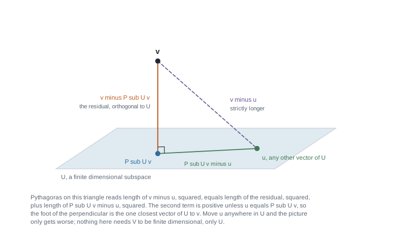
The figure is the proof, not an illustration of it. The vertical leg is the residual, meeting the plane at a right angle because the lemma put it in \(U^{\perp}\); the horizontal leg \(P_U v - u\) lies in the plane; the dashed hypotenuse is \(v - u\). A competing \(u\) moves only the horizontal leg, so it can only lengthen the hypotenuse, and strictly unless that leg has length zero. Notice what the picture does not require: the plane must be finite-dimensional, the space around it need not be.

The number \(\lVert v - P_U v \rVert\) is the distance from \(v\) to \(U\), zero exactly when \(v \in U\). And taking \(u = 0\) gives \(\lVert v \rVert^2 = \lVert P_U v \rVert^2 + \lVert v - P_U v \rVert^2\), which is Bessel’s inequality from Week 6 with the missing quantity finally named.

Note

Where finite-dimensionality earns its place. The hypothesis \(\dim U < \infty\) does two jobs: it supplies an orthonormal basis, and through that it makes a nearest vector exist. Without it the infimum can fail to be attained. Let \(V\) be the real sequences with finitely many nonzero entries, \(\langle x, y \rangle = \sum_i x_iy_i\); fix \(a = (2^{-1}, 2^{-2}, \dots)\), which is not in \(V\); let \(U = \{x \in V : \sum_i a_ix_i = 0\}\). For \(v = e_1\) the distance to \(U\) is \(\sqrt{3}/2\), but nothing in \(U\) attains it: the only candidate is \(e_1 - \tfrac{3}{2}a\), whose nonzero entries never stop. Confirming that infimum needs a density argument in the completion of \(V\), a step compressed here.

Projections as operators, and the converse

Read \(P_U\) as a map \(V \to V\) and it becomes an operator with a short list of properties that characterise it completely.

Theorem. Let \(U\) be a finite-dimensional subspace of an inner product space \(V\) over \(\mathbb{R}\) or \(\mathbb{C}\). Then \(P_U \in \mathcal{L}(V)\) and: (i) \(P_U u = u\) for every \(u \in U\), hence \(P_U^2 = P_U\); (ii) \(\operatorname{im} P_U = U\) and \(\ker P_U = U^{\perp}\); (iii) \(\langle P_U v, w \rangle = \langle v, P_U w \rangle\) for all \(v, w \in V\).

Argument. Linearity is immediate, since \(v \mapsto \langle v, e_i \rangle\) is linear in its first slot and the \(e_i\) are fixed. For (i), expand \(u = \sum_j a_j e_j\); orthonormality gives \(\langle u, e_i \rangle = a_i\), so \(P_U u = u\), and applying this to \(u = P_U v\) yields \(P_U^2 = P_U\). For (ii), \(\operatorname{im} P_U \subseteq U\) by construction and \(\supseteq\) follows from (i); and \(P_U v = 0\) exactly when every \(\langle v, e_i \rangle\) vanishes, which by the expansion argument in the lemma says \(v \in U^{\perp}\). For (iii), write \(w = P_U w + (w - P_U w)\) and use \(P_U v \in U\) with \(w - P_U w \in U^{\perp}\) to get \(\langle P_U v, w \rangle = \langle P_U v, P_U w \rangle\); splitting \(v\) the same way gives \(\langle v, P_U w \rangle = \langle P_U v, P_U w \rangle\).

Property (iii) is self-adjointness. Week 8 defines the adjoint \(T^{*}\) properly and proves it exists and is unique when \(V\) is finite-dimensional; until then the identity is used in the raw form just proved, which needs no such theorem. Item (ii) also assembles into \(V = U \oplus U^{\perp}\) — the internal direct sum of Week 1, produced canonically rather than by choosing a complement — but the systematic treatment of \(U^{\perp}\) waits for Week 8.

Theorem (converse). Let \(V\) be a finite-dimensional inner product space over \(\mathbb{R}\) or \(\mathbb{C}\) and let \(P \in \mathcal{L}(V)\) satisfy \(P^2 = P\) and \(\langle Pv, w \rangle = \langle v, Pw \rangle\) for all \(v, w\). Then \(P = P_U\) for \(U = \operatorname{im} P\).

Argument. \(U = \operatorname{im} P\) is a subspace of the finite-dimensional \(V\), hence finite-dimensional, so \(P_U\) exists. First, \(P\) fixes \(U\) pointwise: any \(u \in U\) is \(Pz\), and \(Pu = P^2z = Pz = u\). Now for any \(v \in V\) and \(u \in U\), \[\langle v - Pv,\, u \rangle = \langle v - Pv,\, Pu \rangle = \langle P(v - Pv),\, u \rangle = \langle Pv - P^2 v,\, u \rangle = 0 ,\] using \(Pu = u\), then self-adjointness, then \(P^2 = P\). So \(v - Pv \in U^{\perp}\) while \(Pv \in U\), and the uniqueness corollary identifies \(Pv\) as \(P_U v\).

Both hypotheses are needed. Dropping self-adjointness gives the oblique projections of the second worked example; dropping idempotence gives, for instance, twice an orthogonal projection, which is self-adjoint but fails to fix \(U\) pointwise — it sends each \(u \in U\) to \(2u\), so \((2P_U)^2 = 4P_U \ne 2P_U\) and no vector outside the kernel is a nearest point of \(U\).

From orthogonality to the normal equations

Everything above is basis-free apart from the orthonormal basis inside the formula. Now put the picture in coordinates in \(F^m\) with the standard inner product, because that is where least squares lives. Nothing new is proved here; the theorems get translated into matrices.

The projection matrix of a full-column-rank array

Let \(A\) be \(m \times k\) real and \(U = \operatorname{col}(A) \subseteq \mathbb{R}^m\), of dimension \(\operatorname{rank} A\). That subspace is finite-dimensional whatever \(A\) is, so \(P_U\) exists; the question is whether a closed formula for it does.

Lemma. \(A^{\mathsf{T}}A\) is invertible if and only if the columns of \(A\) are independent, that is, \(\operatorname{rank} A = k\).

Argument. Suppose the columns are independent and \(A^{\mathsf{T}}Ax = 0\). Multiply on the left by \(x^{\mathsf{T}}\): \(0 = x^{\mathsf{T}}A^{\mathsf{T}}Ax = (Ax)^{\mathsf{T}}(Ax) = \lVert Ax \rVert^2\), so \(Ax = 0\) by positive-definiteness, so \(x = 0\) by independence. A \(k \times k\) matrix with trivial kernel has rank \(k\) by rank-nullity from Week 3, hence is invertible. Conversely, dependent columns give \(x \ne 0\) with \(Ax = 0\), and then \(A^{\mathsf{T}}Ax = 0\).

Theorem. If the \(m \times k\) real matrix \(A\) has independent columns, then \(P = A(A^{\mathsf{T}}A)^{-1}A^{\mathsf{T}}\) is the matrix, relative to the standard basis, of the orthogonal projection of \(\mathbb{R}^m\) onto \(\operatorname{col}(A)\).

Argument. Write \(G = A^{\mathsf{T}}A\), invertible by the lemma. Idempotence: \(P^2 = AG^{-1}(A^{\mathsf{T}}A)G^{-1}A^{\mathsf{T}} = AG^{-1}A^{\mathsf{T}} = P\). Symmetry: \(G^{\mathsf{T}} = G\), so \((G^{-1})^{\mathsf{T}} = G^{-1}\) and \(P^{\mathsf{T}} = P\). Image: every output is \(A\) times something, and \(P(Ax) = AG^{-1}Gx = Ax\), so \(P\) fixes \(\operatorname{col}(A)\) pointwise and \(\operatorname{im} P = \operatorname{col}(A)\). Symmetry of the array gives \(\langle Pv, w \rangle = (Pv)^{\mathsf{T}}w = v^{\mathsf{T}}P^{\mathsf{T}}w = \langle v, Pw \rangle\), so the converse theorem applies.

One hypothesis in that last step is easy to lose. A symmetric matrix corresponds to a self-adjoint operator only when the basis it is written in is orthonormal, and the argument used the standard basis of \(\mathbb{R}^m\), orthonormal for the dot product; in a skewed basis the same operator generally has a non-symmetric array. Over \(\mathbb{C}\) everything holds with \(A^{*}\) for \(A^{\mathsf{T}}\), and \(x^{*}A^{*}Ax = \lVert Ax \rVert^2\) is where the conjugate is required.

Least squares as projection onto the column space

Given \(A\) of size \(m \times k\) and \(b \in \mathbb{R}^m\), minimise \(\lVert b - Ax \rVert\) over \(x \in \mathbb{R}^k\). As \(x\) ranges over \(\mathbb{R}^k\), the vector \(Ax\) ranges over exactly \(\operatorname{col}(A)\), so the problem splits. Which vector of \(\operatorname{col}(A)\) is nearest \(b\)? Exactly one, namely \(P_U b\) with \(U = \operatorname{col}(A)\), by best approximation. Which \(x\) produce it? The solution set of \(Ax = P_U b\), a consistent system by construction.

So a minimiser always exists, whatever \(A\) and \(b\) are; the minimum value \(\lVert b - P_U b \rVert\) is unique; and \(\hat{x}\) is unique exactly when the columns of \(A\) are independent, since two minimisers differ by a member of \(\ker A\).

To get equations you can solve, avoid the projection matrix. The vector \(\hat{x}\) minimises precisely when \(A\hat{x} = P_U b\), precisely when \(b - A\hat{x} \in U^{\perp}\) by the uniqueness corollary, precisely when \(b - A\hat{x}\) is orthogonal to each column of \(A\). Stacking those \(k\) conditions is the single statement \(A^{\mathsf{T}}(b - A\hat{x}) = 0\), since the \(i\)-th entry of \(A^{\mathsf{T}}z\) is the dot product of the \(i\)-th column with \(z\). Rearranged, \[A^{\mathsf{T}}A\,\hat{x} = A^{\mathsf{T}}b ,\] the normal equations — derived, not posited, and “normal” in the geometric sense of perpendicular. Nothing was inverted, so these equations are consistent for every \(A\) and \(b\); independence of the columns is needed only to make the minimiser unique, and only then may you write \(\hat{x} = (A^{\mathsf{T}}A)^{-1}A^{\mathsf{T}}b\).

Worked example — fitting a line to four data pairs

Fit a line \(y = c + mx\) to the pairs \((0, 1)\), \((1, 3)\), \((2, 4)\), \((3, 4)\) in the least-squares sense, over \(\mathbb{R}\) with the standard inner product on \(\mathbb{R}^4\).

Step 1. Write the system. Demanding \(c + mx_i = y_i\) for each pair gives \(Ax = b\) with \[A = \begin{pmatrix} 1 & 0 \\ 1 & 1 \\ 1 & 2 \\ 1 & 3 \end{pmatrix}, \qquad x = \begin{pmatrix} c \\ m \end{pmatrix}, \qquad b = \begin{pmatrix} 1 \\ 3 \\ 4 \\ 4 \end{pmatrix} .\] Neither column is a scalar multiple of the other, so \(\operatorname{rank} A = 2\) and \(\operatorname{col}(A)\) is a plane inside \(\mathbb{R}^4\). The lemma therefore makes \(A^{\mathsf{T}}A\) invertible and \(\hat{x}\) unique.

Step 2. Form the normal equations. The entries of \(A^{\mathsf{T}}A\) are dot products of columns: the first with itself is \(1 + 1 + 1 + 1 = 4\); the first with the second is \(0 + 1 + 2 + 3 = 6\); the second with itself is \(0 + 1 + 4 + 9 = 14\). The entries of \(A^{\mathsf{T}}b\) are the columns against \(b\): \(1 + 3 + 4 + 4 = 12\) and \(0 \cdot 1 + 1 \cdot 3 + 2 \cdot 4 + 3 \cdot 4 = 23\). So \[\begin{pmatrix} 4 & 6 \\ 6 & 14 \end{pmatrix}\begin{pmatrix} c \\ m \end{pmatrix} = \begin{pmatrix} 12 \\ 23 \end{pmatrix} .\]

Step 3. Solve exactly. The determinant is \(4 \cdot 14 - 6 \cdot 6 = 56 - 36 = 20 \ne 0\), and inverting a two-by-two array by its adjugate, \[\hat{x} = \frac{1}{20}\begin{pmatrix} 14 & -6 \\ -6 & 4 \end{pmatrix}\begin{pmatrix} 12 \\ 23 \end{pmatrix} = \frac{1}{20}\begin{pmatrix} 168 - 138 \\ -72 + 92 \end{pmatrix} = \frac{1}{20}\begin{pmatrix} 30 \\ 20 \end{pmatrix} = \begin{pmatrix} 3/2 \\ 1 \end{pmatrix} .\] The fitted line is \(y = \tfrac{3}{2} + x\). Check the equations directly rather than trusting the inverse: \(4 \cdot \tfrac{3}{2} + 6 = 12\) and \(6 \cdot \tfrac{3}{2} + 14 = 23\). Both hold.

Step 4. The projection and the residual. Evaluating \(\tfrac{3}{2} + x\) at \(x = 0, 1, 2, 3\) gives \(A\hat{x} = \big(\tfrac{3}{2}, \tfrac{5}{2}, \tfrac{7}{2}, \tfrac{9}{2}\big)^{\mathsf{T}}\), which is \(P_U b\). Subtracting, \[r = b - A\hat{x} = \begin{pmatrix} 1 - 3/2 \\ 3 - 5/2 \\ 4 - 7/2 \\ 4 - 9/2 \end{pmatrix} = \begin{pmatrix} -1/2 \\ 1/2 \\ 1/2 \\ -1/2 \end{pmatrix} .\] Since \(r \ne 0\), no line meets all four pairs and the original system was indeed inconsistent.

The fitted line and the four vertical gaps it leaves behind.

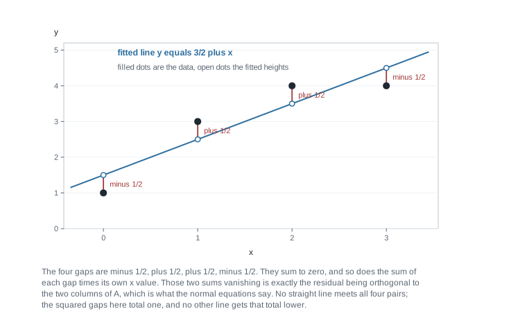
The figure draws the four gaps as vertical segments, which is what “least squares” minimises: not perpendicular distance to the drawn line in the plane of the picture, but the sum of the squares of those four signed vertical lengths, \(4 \cdot \tfrac{1}{4} = 1\). That all four gaps have the same magnitude \(\tfrac{1}{2}\) is a feature of this data; that the upward ones balance the downward ones is not — it is the first of the two cancellations checked next, forced by the constant column of \(A\).

Step 5. Verify orthogonality against both columns. Against \((1,1,1,1)^{\mathsf{T}}\): \(-\tfrac{1}{2} + \tfrac{1}{2} + \tfrac{1}{2} - \tfrac{1}{2} = 0\). Against \((0,1,2,3)^{\mathsf{T}}\): \(0 + \tfrac{1}{2} + 1 - \tfrac{3}{2} = 0\). So \(A^{\mathsf{T}}r = 0\), and since the columns span \(\operatorname{col}(A)\), the residual is orthogonal to the whole plane.

Step 6. Pythagoras as a numerical check. The theorem predicts \(\lVert b \rVert^2 = \lVert A\hat{x} \rVert^2 + \lVert r \rVert^2\). Here \(\lVert b \rVert^2 = 1 + 9 + 16 + 16 = 42\), \(\lVert A\hat{x} \rVert^2 = \tfrac{9 + 25 + 49 + 81}{4} = \tfrac{164}{4} = 41\), and \(\lVert r \rVert^2 = 4 \cdot \tfrac{1}{4} = 1\). And \(41 + 1 = 42\).

The vector b outside the column space, its projection inside, and this example’s numbers.

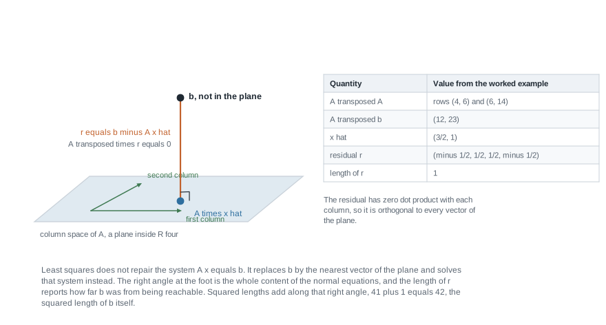
The figure gathers the computation into one picture: the plane is \(\operatorname{col}(A)\) inside \(\mathbb{R}^4\), the two arrows are its spanning columns, \(b\) sits off it, and the right angle at the foot is the content of Step 5. The table beside it lists the numbers above, so geometry and arithmetic can be read against each other.

This establishes that \(y = \tfrac{3}{2} + x\) uniquely minimises the sum of squared vertical gaps, with minimum \(1\). It does not establish that the line is correct, or that the data came from a line: least squares reports the nearest vector in a subspace you chose. On the field, every number above lies in \(\mathbb{Q}\), so the computation runs verbatim over the rationals; the distance \(\lVert r \rVert\) generally does not, and is \(1\) here only by luck.

The same reasoning, transferred

Run the same argument on a plane in \(\mathbb{R}^3\), using an orthonormal basis instead of the normal equations. Let \(U = \{(x, y, z) \in \mathbb{R}^3 : x + y + z = 0\}\), of dimension two, and \(v = (3, 0, 0)\). Take \(u_1 = (1, -1, 0)\) and \(u_2 = (1, 1, -2)\), both in \(U\) since their entries sum to zero, and orthogonal since \(1 - 1 + 0 = 0\). Their lengths are \(\sqrt{2}\) and \(\sqrt{6}\), so \(e_1 = \tfrac{1}{\sqrt{2}}(1,-1,0)\) and \(e_2 = \tfrac{1}{\sqrt{6}}(1,1,-2)\) form an orthonormal basis. Then \(\langle v, e_1 \rangle = 3/\sqrt{2}\), \(\langle v, e_2 \rangle = 3/\sqrt{6}\), and \[P_U v = \tfrac{3}{2}(1,-1,0) + \tfrac{1}{2}(1,1,-2) = (2, -1, -1) .\] Its entries sum to zero, so it lies in \(U\). The residual is \((3,0,0) - (2,-1,-1) = (1,1,1)\), a multiple of the plane’s normal direction — as it must be, since \(U^{\perp}\) is the line spanned by \((1,1,1)\). Pythagoras checks: \(9 = 6 + 3\).

What stayed the same: the residual is orthogonal to the subspace, the projection is the unique nearest vector, squared lengths add. What changed: the route. The line fit went through the normal equations because no orthonormal basis of \(\operatorname{col}(A)\) was in hand; here Week 6 supplied one directly and nothing had to be inverted. Notice too that the basis involved \(\sqrt{2}\) and \(\sqrt{6}\) while \(P_U v\) has integer entries — the irrationalities cancel, because the projection depends only on \(U\).

Second worked example — an idempotent that is not self-adjoint

Work in \(\mathbb{R}^2\) with the dot product, and let \[P = \begin{pmatrix} 1 & 1 \\ 0 & 0 \end{pmatrix}, \qquad Q = \begin{pmatrix} 1 & 0 \\ 0 & 0 \end{pmatrix} .\]

Both are idempotent. For \(P\): row one, column one of \(P^2\) is \(1 \cdot 1 + 1 \cdot 0 = 1\); row one, column two is \(1 \cdot 1 + 1 \cdot 0 = 1\); the second row vanishes because the second row of the left factor does. So \(P^2 = P\), and for \(Q\) the check is immediate.

Both have the same image. Both columns of \(P\) are \((1,0)^{\mathsf{T}}\), so \(\operatorname{im} P\) is the horizontal axis \(U = \operatorname{span}\{(1,0)\}\), and \(Q\) gives the same \(U\). Image alone does not tell them apart.

They differ in their kernels. \(P(a,b)^{\mathsf{T}} = (a + b, 0)^{\mathsf{T}}\) vanishes exactly when \(a + b = 0\), so \(\ker P = \operatorname{span}\{(1,-1)\}\), the line of slope \(-1\). But \(Q(a,b)^{\mathsf{T}} = (a,0)^{\mathsf{T}}\), so \(\ker Q = \operatorname{span}\{(0,1)\} = U^{\perp}\). An idempotent operator projects onto its image along its kernel, and only \(Q\) projects along the perpendicular.

Only \(Q\) is self-adjoint. \(P^{\mathsf{T}}\) has rows \((1,0)\) and \((1,0)\), which is not \(P\). Concretely, with \(v = (0,1)^{\mathsf{T}}\) and \(w = (1,0)^{\mathsf{T}}\), \(\langle Pv, w \rangle = \langle (1,0), (1,0) \rangle = 1\) while \(\langle v, Pw \rangle = \langle (0,1), (1,0) \rangle = 0\). Property (iii) fails, and since the converse theorem is an equivalence, \(P\) cannot be an orthogonal projection.

The best-approximation property fails, measurably. Take \(v = (1,2)^{\mathsf{T}}\). Then \(Pv = (3,0)^{\mathsf{T}}\) and \(Qv = (1,0)^{\mathsf{T}}\), both on \(U\), with \(\lVert v - Pv \rVert = \lVert (-2,2) \rVert = 2\sqrt{2}\) and \(\lVert v - Qv \rVert = \lVert (0,2) \rVert = 2\). Since \(2 < 2\sqrt{2}\), the vector \(Pv\) is not nearest, while \(Qv\) is by best approximation applied to \(U\) with orthonormal basis \(\{(1,0)\}\). Note also that \(v - Pv = (-2,2)\) is a multiple of \((1,-1)\), confirming that \(P\) slid \(v\) along its own kernel.

One vector, one target line, two idempotent operators, two different landing places.

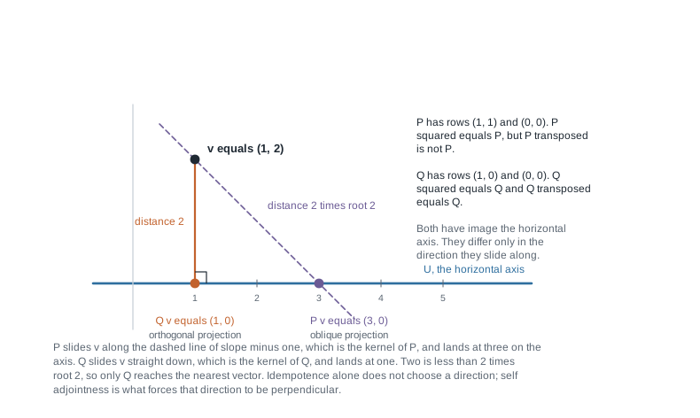
The figure sets the two routes side by side: the dashed slanted path is \(P\) sliding along its kernel to land at \(3\) on the axis, the vertical path is \(Q\) dropping perpendicular to land at \(1\), and the labelled distances are the numbers just computed. Idempotence fixes only the destination subspace, never the direction of travel; self-adjointness pins the direction down. Oblique projections are still useful — they decompose a space along a chosen pair of complementary subspaces, in the sense of Week 1 — they simply do not minimise distance.

The misreading to avoid

The misreading: least squares finds the solution set of an inconsistent system. Stated that way it contradicts itself. If \(Ax = b\) is inconsistent then no \(x\) satisfies it, the set of those that do is empty, and no procedure can return a member of an empty set. Least squares never touches that set. It solves a different problem — minimise \(\lVert b - Ax \rVert\) — whose feasible set is all of \(\mathbb{R}^k\) and which therefore always has a minimiser. The two problems agree when \(b \in \operatorname{col}(A)\), since then the minimum is zero, which is why the substitution feels harmless and is not.

The practical damage is that the substitution hides the residual, and the residual is the only honest report of what the model could not reproduce. In the worked example \(\lVert r \rVert = 1\); that number, not \(\hat{x}\), is what says the four pairs are not collinear. The same confusion invites a second inference — that a smaller residual means a better model — when a larger subspace always gives a residual at least as small. Fitting a cubic to four pairs drives the residual to zero and explains nothing, because four independent columns make the column space all of \(\mathbb{R}^4\) and \(b\) is already in it.

A companion misreading is that any \(P\) with \(P^2 = P\) is the projection onto its image, so best approximation applies. The second worked example gives two idempotents with the same image and different kernels, and only the self-adjoint one minimises distance. Meeting an idempotent operator, ask which subspace it projects onto and which subspace it projects along, and only then decide whether “orthogonal” applies.

One more distinction saves grief later. The normal equations are consistent even when \(A\) has dependent columns, since the derivation used only that \(P_U b\) lies in \(\operatorname{col}(A)\). Dependence destroys the uniqueness of \(\hat{x}\), not the existence of a nearest vector. With columns \((1,1,1)^{\mathsf{T}}\) and \((2,2,2)^{\mathsf{T}}\) and \(b = (1,1,4)^{\mathsf{T}}\), the normal equations reduce to \(c + 2m = 2\), a whole line of minimisers, every one producing the same \(A\hat{x} = (2,2,2)^{\mathsf{T}}\). The projection is well defined; the coefficients are not.

Practice on your own

These are for your own checking rather than for submission, and each is within reach of Weeks 5 through 7.

1. A second line fit. Fit \(y = c + mx\) by least squares to \((1,1)\), \((2,2)\), \((3,2)\), \((4,5)\). Form \(A^{\mathsf{T}}A\) and \(A^{\mathsf{T}}b\), solve with exact fractions, compute the residual, and verify it is orthogonal to both columns. Then check the Pythagorean relation among the squared lengths of \(b\), \(A\hat{x}\), and the residual.
2. Projection onto a plane, two ways. Let \(U \subseteq \mathbb{R}^3\) be spanned by \((1,0,1)\) and \((0,1,1)\), and \(v = (2,0,0)\). Compute \(P_U v\) once by running Gram-Schmidt and applying the projection formula, once by forming \(A(A^{\mathsf{T}}A)^{-1}A^{\mathsf{T}}\). Confirm they agree, and name the hypothesis each route needed.
3. A projection in a function space. In \(C[0,1]\) with \(\langle f, g \rangle = \int_0^1 fg\), let \(U\) be the constant functions, with \(\{1\}\) as an orthonormal basis. Compute \(P_U f\) for \(f(x) = x^2\) and verify that \(f - P_U f\) is orthogonal to every constant. Here \(V\) is infinite-dimensional and \(U\) is not: locate the hypothesis of the best-approximation theorem doing the work.
4. Idempotents, catalogued. Find every \(2 \times 2\) real matrix \(P\) with \(P^2 = P\) and \(\operatorname{rank} P = 1\). Describe the family by its image line and its kernel line, prove that exactly one member for each image line is symmetric, and say in a sentence why that matches the converse theorem.
5. Where the inverse is not allowed. Give a \(3 \times 2\) real matrix \(A\) of rank one and a vector \(b\) outside \(\operatorname{col}(A)\). Show \(A^{\mathsf{T}}A\) is singular, exhibit two distinct minimisers \(\hat{x}\), and show they produce the same \(A\hat{x}\). State which theorem on this page guarantees that agreement.

Where to read more

A second treatment in another voice often settles a theorem that a first reading only moved. The three addresses below are offered online at no cost by their providers; availability and licence terms are as those providers state them, and neither is confirmed here.

• MIT OpenCourseWare 18.06 Linear Algebra — the closest computational match: projections onto subspaces, projection matrices, and least squares in coordinates.
• MIT OpenCourseWare 18.700 Linear Algebra — the proof-based counterpart, developing the orthogonal decomposition and best approximation before any matrix appears.
• Linear Algebra Done Wrong by Sergei Treil — an abstract-first text whose inner product chapter treats orthogonal projection and the normal equations in the order used here.
• The optional Roman alignment for this week is the chapter on inner product spaces, in the section on orthogonal projections, with the sections on orthogonal sets carried over from Week 6. That text is an optional reference: a borrowed or library copy suffices, and nothing from it is reproduced here.
• Course pages: the notes overview, the syllabus, the schedule, and the resources page. The learning management system remains authoritative for section logistics and graded details.

Where this goes next

This week leaned on \(U^{\perp}\) constantly and defined it only in passing. Two facts about it were needed everywhere — that a vector orthogonal to a spanning set of \(U\) is orthogonal to all of \(U\), and that \(U \cap U^{\perp} = \{0\}\) — and both were proved where they were used. The decomposition \(V = U \oplus U^{\perp}\) fell out as a by-product, a poor way to treat the first canonical direct sum the course has produced.

Week 8, on orthogonal complements, adjoints, and the four fundamental subspaces, makes the repair. It proves \(\dim U + \dim U^{\perp} = \dim V\) and \((U^{\perp})^{\perp} = U\) for finite-dimensional \(U\), and constructs the adjoint \(T^{*}\) properly, so the self-adjointness identity used here becomes an equation between operators. It also settles the hypothesis flagged above: the matrix of \(T^{*}\) is the conjugate transpose of the matrix of \(T\) relative to an orthonormal basis. Looking back instead: Week 6 supplies the Gram-Schmidt process every projection formula here depends on, Week 5 carries the Pythagorean identity that proves best approximation, and the notes index and course home page list what is here.