Week 11 — Robust regression ideas

One point can steer a least-squares line, and what to do about it

Source basis. Original instructor-authored notes; data is synthetic (40 clean points plus one contaminating point from a fixed generator, seed 45211). Open texts are conceptual companions cited by section title only (map-don’t-mine); no prose, figures, examples, or exercises are reproduced. See Open readings & attribution. Ungraded — Blackboard is authoritative for graded work.

This week. Last week we made summaries resistant: the median and the trimmed mean barely flinch when one point misbehaves. This week we carry the same worry into a relationship. A regression line is a summary too — a summary of how y moves with x — and it can be steered by a single point far more easily than a mean can. We will watch one point swing a least-squares line, meet a resistant fit that refuses to follow it, and learn to see influence before it fools us.

Learning goals

By the end of this week you should be able to:

Explain why ordinary least squares (OLS) is sensitive to a point that is extreme in x (high leverage) and off the trend (large residual), and why that combination is what does the damage.
Describe the idea of a resistant regression (a Huber M-estimator / least-trimmed-squares) that down-weights points the OLS line would chase.
Read a leverage-vs-residual diagnostic and a Cook’s distance to locate an influential point rather than guess.
State plainly why “robust regression has no assumptions” is false, and why no single number — slope or $R^2$ — is trustworthy without an influence check.

Where we are

Least squares chooses the line that minimizes the sum of squared vertical residuals. Squaring is the whole story of its fragility: a point twice as far from the line contributes four times the penalty, so OLS will bend a long way to shrink one big residual. A point that is also far out in x has extra pull — moving the line near that point barely disturbs the fit near the crowded middle. That leverage is measured by the hat value $h_{ii}$ , the $i$ -th diagonal of the projection (“hat”) matrix $H = X(X^\top X)^{-1}X^\top$ ; it depends only on the x-values, and a common flag is $h_{ii} > 2p/n$ .

Our running example is a synthetic scatter: 40 points with a genuine linear trend ( $y = 3 + 1.2\,x + \text{noise}$ ), plus one contaminating point at $(19, 7)$ sitting far to the right and well below the trend. That one point is a high-leverage, large-residual troublemaker — exactly the kind least squares cannot resist.

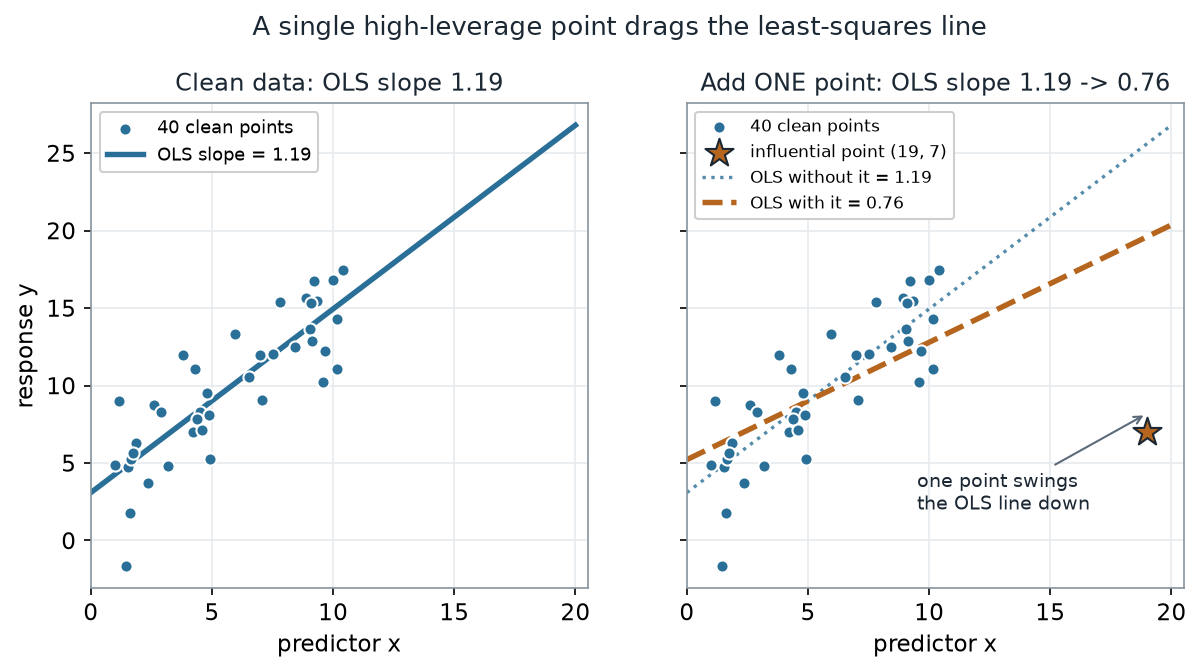
Two scatterplots side by side. Left: 40 clean points with a teal least-squares line of slope 1.19. Right: the same points plus one star-marked influential point at x=19, y=7 far to the lower right; the dotted line shows the original slope 1.19 and a dashed ochre line shows the refit slope 0.76, visibly flatter, pulled down toward the star.

What to notice. Nothing about the 40 original points changed. One point — placed far out in x and off the line — dragged the least-squares slope from 1.19 down to 0.76. The line rotates toward the star because chasing that single large residual buys OLS a big reduction in squared error. This is the core hazard: with least squares, influence is not democratic.

The fits, as numbers (nonvisual equivalent).

Fit	Slope	Intercept	$R^2$
OLS, 40 clean points	1.19	3.09	0.706
OLS, + the point $(19,7)$	0.76	5.22	0.411
True generating line	1.20	3.00	—

The R you would run computes the two fits — and note there is no plotting in it; the picture is a downstream artifact:

# Schematic: the named data objects are the sample(s) described in the text above; this illustrates the analysis, not a self-contained runnable block.
# ordinary least squares, before and after adding the one point
fit_clean <- lm(y ~ x, data = clean)          # slope ~ 1.19
fit_all   <- lm(y ~ x, data = contaminated)   # slope ~ 0.76

coef(fit_clean); coef(fit_all)                # compare the slopes
summary(fit_all)$r.squared                    # 0.41 — lower, not higher

Worked example — a resistant fit that refuses to follow

If the trouble is that OLS treats every point as equally worthy of being chased, the fix is to let the data earn its weight. A Huber M-estimator (the default of MASS::rlm in R) does exactly this: it fits the line by iteratively re-weighting each point according to how large its residual is, on a robust scale. Points inside a band count fully; points outside it — like our star — count less and less.

Concretely, the algorithm starts from the OLS fit, estimates a robust residual scale $s$ from the median absolute deviation, forms weights $w_i = \min\!\big(1,\; k / |r_i / s|\big)$ with the standard tuning constant $k = 1.345$ , refits by weighted least squares, and repeats until the line stops moving.

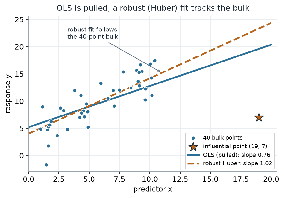
Scatterplot of the 40 bulk points plus the star-marked influential point at x=19, y=7. A teal solid least-squares line of slope 0.76 is pulled toward the star; a dashed ochre robust Huber line of slope 1.02 stays with the 40-point bulk, passing through the crowd of points.

What to notice. The robust line does not delete the odd point — it discounts it. Because the star’s residual is huge on the robust scale, its Huber weight falls to about 0.24 (a full-weight point is 1.0), so it can no longer command the fit. The result, slope 1.02, lands near the truth (1.20) that the 40 honest points actually carry. Resistance, not deletion.

OLS vs robust on the contaminated data (nonvisual equivalent).

Fit	Slope	Intercept	Weight on the point $(19,7)$
OLS (least squares)	0.76	5.22	1.00 (implicitly)
Robust Huber, $k = 1.345$	1.02	4.03	0.24

# Schematic: the named data objects are the sample(s) described in the text above; this illustrates the analysis, not a self-contained runnable block.
# a resistant fit: Huber M-estimation, k = 1.345 (MASS::rlm default)
library(MASS)
fit_rob <- rlm(y ~ x, data = contaminated, psi = psi.huber, k = 1.345)

coef(fit_rob)                 # slope ~ 1.02, back near the truth
fit_rob$w[which.max(x)]       # the huge-x point earns a small weight (~0.24)

Locating the culprit: a leverage-vs-residual diagnostic

You will not always know which point is the problem, and with many predictors you cannot simply eyeball the scatter. The workhorse diagnostic plots each point’s leverage $h_{ii}$ against its studentized residual, and scales the marker by Cook’s distance — a single number that combines “how far out in x” with “how far off the line,” measuring how much the whole fit would move if that point were dropped.

Scatterplot of leverage on the x-axis versus studentized residual on the y-axis for 41 points. Forty teal points cluster at low leverage (below 0.07) with residuals between about -2.4 and 1.3. One ochre star sits far to the lower right at leverage 0.32 and residual -4.4, with a much larger marker indicating a Cook's distance of 4.7. A dashed vertical line marks the 2p/n leverage rule at 0.098. — Scatterplot of leverage on the x-axis versus studentized residual on the y-axis for 41 points. Forty teal points cluster at low leverage (below 0.07) with residuals between about -2.4 and 1.3. One ochre star sits far to the lower right at leverage 0.32 and residual -4.4, with a much larger marker indicating a Cook’s distance of 4.7. A dashed vertical line marks the 2p/n leverage rule at 0.098.

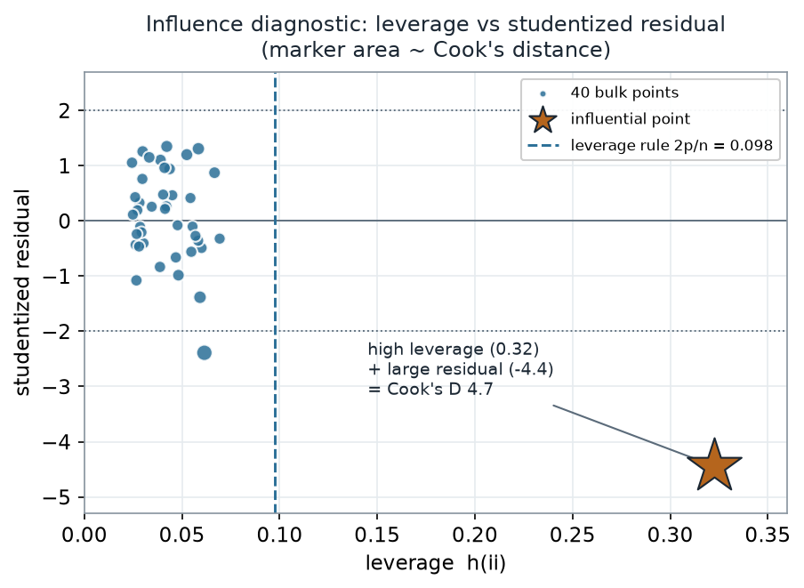
What to notice. The troublemaker separates on both axes at once. Its leverage (0.32) is more than three times the $2p/n = 0.098$ rule-of-thumb line and far beyond the bulk’s largest (0.069); its studentized residual (−4.4) is well past the $\pm 2$ guides. One bulk point does dip past the $-2$ guide — studentized residual −2.4 at $x\approx1.5$ — yet its leverage stays low (0.06), so its Cook’s $D$ is only 0.19: a big residual alone, without leverage, is not influence. Cook’s distance fuses the star’s two extremes into 4.7, roughly 25 times any other point’s. The diagnostic does not tell you to delete the point — it tells you where to look.

Diagnostic read-out (nonvisual equivalent).

Quantity	Influential point	Largest among the other 40
Leverage $h_{ii}$ (flag at $2p/n = 0.098$ )	0.323	0.069
Studentized residual	−4.44	−2.4 in size (low leverage, at $x\approx1.5$ )
Cook’s distance	4.70	0.19

# Schematic: the named data objects are the sample(s) described in the text above; this illustrates the analysis, not a self-contained runnable block.
# influence diagnostics from the (contaminated) least-squares fit
h     <- hatvalues(fit_all)      # leverage; flag h > 2 * 2 / n
rstud <- rstandard(fit_all)      # studentized residuals
cooks <- cooks.distance(fit_all) # Cook's distance combines both

which.max(cooks)                 # points straight at the one troublemaker

A common mistake

“The regression gave me a slope and an $R^2$ — those are the numbers, so I report them.” A single summary is only as trustworthy as the influence behind it. Here, one point dragged the slope from 1.19 to 0.76 and tanked $R^2$ from 0.71 to 0.41, so an analyst reading $R^2$ alone would wrongly conclude that x is a weak predictor — when the 40 honest points carry a solid relationship. And note the partner myth: a robust fit is resistant, not assumption-free. It still assumes the bulk of the data shares one linear trend with roughly symmetric errors; hand it two genuine sub-populations and it will happily fit a line through neither. Robustness buys you resistance to a few bad points, not permission to skip thinking.

A two-panel diagram. Left panel titled THE MYTH shows R-squared = 0.41 in large type with the quote 'R-squared is only 0.41 so x is a weak predictor, and the slope is 0.76 — report the numbers.' An arrow points right to THE REALITY panel listing: in the 40-point bulk R-squared = 0.71 a solid relationship; one point tanked R-squared to 0.41 and swung the slope 1.19 to 0.76; its Cook's distance is 4.7 versus 0.19 for every other point; a robust fit recovers 1.02, resistant not assumption-free. — A two-panel diagram. Left panel titled THE MYTH shows R-squared = 0.41 in large type with the quote ‘R-squared is only 0.41 so x is a weak predictor, and the slope is 0.76 — report the numbers.’ An arrow points right to THE REALITY panel listing: in the 40-point bulk R-squared = 0.71 a solid relationship; one point tanked R-squared to 0.41 and swung the slope 1.19 to 0.76; its Cook’s distance is 4.7 versus 0.19 for every other point; a robust fit recovers 1.02, resistant not assumption-free.

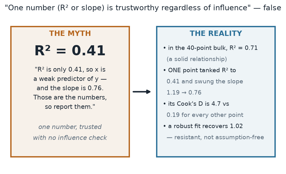
What to notice. The same experiment sends two “one-number” readings in opposite directions: the slope fell (1.19 → 0.76) and $R^2$ fell (0.71 → 0.41), so a slope-watcher and an $R^2$ -watcher would draw different-but-both-wrong conclusions from the very same contaminated fit. Only the influence check — one point with Cook’s distance 4.7 against a field maximum of 0.19 — reconciles them and points to the fix.

Myth vs. reality, as numbers (nonvisual equivalent).

Reading	The number alone	What the influence check adds
$R^2$	0.41 (“weak”)	0.71 in the 40-point bulk; one point tanked it
OLS slope	0.76	true 1.20; robust fit recovers 1.02
Influence	(unseen)	Cook’s D 4.7 vs 0.19 for every other point

Check your understanding (ungraded)

In your own words, what two properties must a point have to swing a least-squares line, and why does a point that is extreme in x but on the trend do little harm?
The Huber fit gave the point $(19,7)$ a weight near 0.24 instead of dropping it. Contrast “down-weighting” with “deleting the outlier” — what does the robust approach keep that deletion throws away?
Adding one point lowered $R^2$ from 0.71 to 0.41 here. Describe a different placement of a single high-leverage point that would instead make $R^2$ look artificially high. What does that tell you about trusting $R^2$ ?
Cook’s distance for the star was about 4.7, versus 0.19 for every other point. If a colleague says “just delete the point with the biggest Cook’s distance,” what should you do first, and why?

Reading guide

OpenIntro Statistics 4e — Outliers in linear regression — a conceptual companion to leverage vs. residual and which “outliers” actually move a line; read for the intuition, then check it against the diagnostic above.
Learning Statistics with R (Navarro) — Regression diagnostics — reinforces hat values, studentized residuals, and Cook’s distance as the standard toolkit (cited, not reproduced).
NIST/SEMATECH e-Handbook — Linear Least Squares Regression — an instructor reference on least squares and how influential observations enter the fit.
IMS — Linear regression with a single predictor — the single-predictor model this week resists; a conceptual map, not a source to mine. Robust estimation itself is an instructor extension beyond these introductory texts.

Accessibility notes

Mathematics is live text ( $h_{ii} = X(X^\top X)^{-1}X^\top$ and $w_i = \min(1, k/|r_i/s|)$ render as MathML, not images). Every figure carries an alt line stating its message, a “what to notice” reading, and an adjacent data-summary table, so each point survives without the picture. Series are distinguished by linestyle and marker (OLS = solid line; robust = dashed line; the influential point = a star marker), never by color alone, and every line is labeled with its slope. A clean lint and a clean render are evidence; the rendered assistive-technology review is a human step.

Assessment (descriptive only)

This week contributes learning evidence toward diagnosing influence in a regression and choosing between a least-squares and a resistant fit for a purpose. That is the shape only; the actual graded prompts, points, and due dates live in Blackboard.

Public vs. graded. These are public, ungraded notes and practice. Graded prompts, keys, rubrics, point values, and due dates live in Blackboard Ultra, which governs.

Looking ahead

Next week we stop treating methods one at a time and put them side by side: the same dataset analyzed by a $t$ -test, a Wilcoxon test, and a bootstrap — first on well-behaved data where they agree, then on skewed, outlier-laden data where they part ways. The habit we are building all term — ask what is fragile, then choose for a purpose — is exactly what tells you which answer to trust when they disagree.