Week 3 — Permutation logic

Testing by relabeling, and what ‘exchangeable under the null’ really licenses

Source basis. Original instructor-authored notes; data is synthetic (two groups of eight “quiz scores” drawn from a fixed generator, seed 45203). Open texts are conceptual companions cited by section title only (map-don’t-mine); no prose, figures, examples, or exercises are reproduced. See Open readings & attribution. Ungraded — Blackboard is authoritative for graded work.

This week. In Weeks 1–2 we asked what is fragile in a sample and met ranks and the ECDF. Now we build our first resampling test. Suppose two groups differ by some amount — is that difference more than the label shuffle could have produced by chance? A permutation test answers it without a table of critical values: it manufactures the null distribution by relabeling the data we already have, then asks how often chance alone beats what we saw.

Learning goals

By the end of this week you should be able to:

• State the exchangeability assumption that a permutation test rests on, and say what it means for the group label to “carry no information” under the null.
• Build a permutation null distribution of a statistic (here, a difference in means) by shuffling the labels and recomputing.
• Compute a two-sided permutation p-value and read it as a proportion of relabelings at least as extreme as the observed value.
• Tell what to permute (the labels, across the whole pool) apart from moves that only look like permuting.

Where we are

Our running example is small on purpose: two sections sit the same quiz, eight students each. Section A scores 63, 66, 67, 68, 70, 71, 79, 85; Section B scores 69, 71, 73, 81, 82, 84, 87, 91. Section B looks stronger — its mean is 79.75 against A’s 71.125, a gap of 8.62 points (79.75 − 71.125 = 8.625, shown rounded) — but with only eight scores a side, a gap like that could easily be luck of the draw. We need a yardstick for “could easily be luck,” and a permutation test builds that yardstick from the data itself.

The one assumption: exchangeability

The null hypothesis here is not “the means are equal” in a vague sense; it is the sharp claim that the group label is irrelevant — every student’s score would have been the same had they been assigned to the other section. If that is true, the sixteen scores are just sixteen scores, and the particular split into “A” and “B” we happened to observe is one of many equally likely splits. That property — that under the null we could permute the labels without changing the joint distribution — is called exchangeability, and it is the entire license for what follows.

So we do exactly that: hold the sixteen values fixed, shuffle the A/B labels, and recompute the difference in means. One shuffle gives one “difference that chance could produce.” Thousands of shuffles trace out the whole range of differences the null can manufacture.

Two rows of the same sixteen score-boxes. The top row is the observed labeling, first eight tagged A and last eight tagged B, with difference in means +8.62. An arrow labeled ‘shuffle the labels’ points down to a second row with the identical sixteen values but the A and B tags reassigned, giving difference +5.62. A caption notes the values are identical in both rows; only the tags moved.

Figure 1: One permutation of the quiz data: the sixteen scores are held fixed; only the A/B labels move. The observed labeling gives a difference of +8.62; this one shuffle happens to give +5.62.

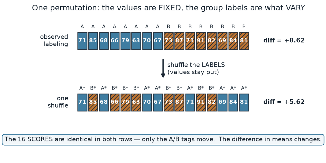
What to notice. Nothing about the numbers changes between the two rows — the same sixteen scores sit in the same sixteen boxes. What changes is only which scores wear the A tag and which wear the B tag, and that alone moves the difference in means from +8.62 to +5.62. Repeat the shuffle many times and the difference wanders; the collection of those wandering differences is the null distribution.

The two groups, as numbers (nonvisual equivalent).

Group	Scores (sorted)	n	Mean
Section A	63, 66, 67, 68, 70, 71, 79, 85	8	71.125
Section B	69, 71, 73, 81, 82, 84, 87, 91	8	79.75
Observed difference mean(B) − mean(A)			+8.62
One illustrative shuffle mean(B*) − mean(A*)			+5.62

Worked example — the permutation test

The statistic is the difference in means, and the observed value is $D_\text{obs} = \bar{x}_B - \bar{x}_A = 8.62$. To judge it, we generate the null distribution by relabeling. Each relabeling draws a fresh assignment of eight “A” and eight “B” tags across the pooled sixteen scores and recomputes $D^{*} = \bar{x}_{B^{*}} - \bar{x}_{A^{*}}$. Ten thousand relabelings give the histogram below.

Histogram of ten thousand relabeled mean differences, roughly bell-shaped and centered at zero, ranging from about minus fifteen to plus fifteen. A solid vertical line marks the observed difference at plus 8.62, out in the right shoulder of the distribution. An annotation notes the null is centered at zero because under the null the label carries no information.

Figure 2: Permutation null distribution of the mean difference over 10,000 relabelings. It is centered at 0 and the observed difference +8.62 sits well out in the right shoulder.

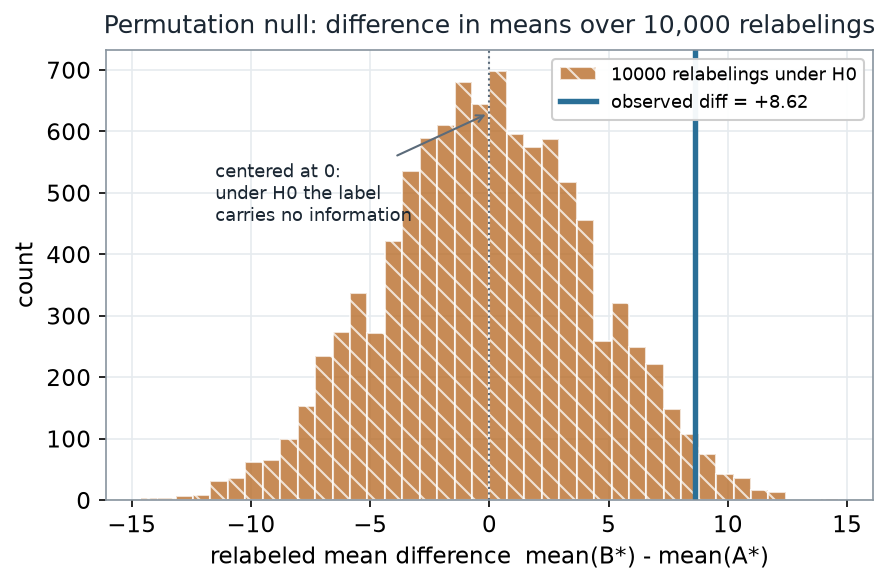
What to notice. The null distribution is centered on zero, not on the observed 8.62 — because when the label genuinely carries no information, positive and negative relabeled differences are equally likely. The observed value is not impossible under the null, but it is uncommon: only a thin slice of relabelings reach out that far. How thin is the p-value.

Permutation null read-out (nonvisual equivalent).

Quantity	Value
Observed difference $D_\text{obs}$	+8.62
Relabelings (B)	10,000
Null center	≈ 0
Relabelings with $|D^{*}| \ge 8.62$	457

The R you would run is short — and notice there is no plotting in it; the picture is downstream:

# two small groups of scores; H0: the group label is exchangeable
set.seed(45203)
scoreA <- c(63, 66, 67, 68, 70, 71, 79, 85)
scoreB <- c(69, 71, 73, 81, 82, 84, 87, 91)

obs    <- mean(scoreB) - mean(scoreA)     # observed difference in means = 8.62
pooled <- c(scoreA, scoreB)               # 16 values, tags set aside
labels <- rep(c("A", "B"), each = 8)

one_diff <- function() {                  # ONE relabeling: shuffle the tags, recompute
  lab <- sample(labels)                   # exchange labels across the WHOLE pool
  mean(pooled[lab == "B"]) - mean(pooled[lab == "A"])
}

B      <- 10000
perm   <- replicate(B, one_diff())        # the permutation null distribution
pval   <- mean(abs(perm) >= abs(obs))     # two-sided p-value ~ 0.046
padd1  <- (1 + sum(abs(perm) >= abs(obs))) / (B + 1)   # the +1 ("add-one") convention

Reading the p-value off the tail

Because “Section B is stronger” and “the sections differ” are different questions, we test two-sided: we count every relabeling whose difference is at least as far from zero as ours in either direction, $|D^{*}| \ge 8.62$. That is the shaded area below.

The same permutation null histogram in grey, with both outer tails beyond plus and minus 8.62 shaded and hatched. Two vertical lines mark plus observed at 8.62 (solid) and minus observed at minus 8.62 (dashed). A boxed label reads: shaded tails, absolute difference at least 8.62, p equals 457 over 10000 equals 0.046.

Figure 3: The two-sided permutation p-value is the shaded tail area: the share of relabelings with $|D^{*}| \ge 8.62$. Here 457 of 10,000, so p ≈ 0.046.

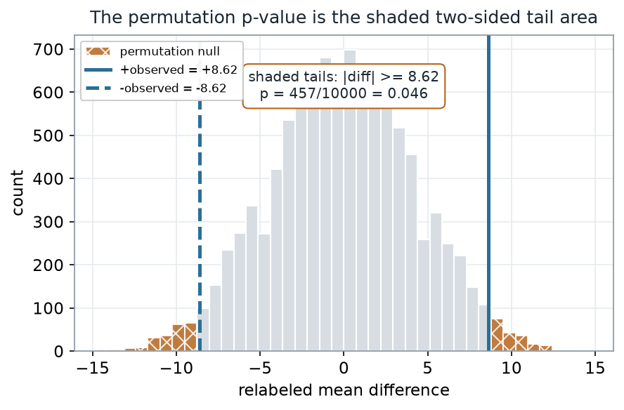
What to notice. The p-value is a counting statement, not a formula: it is the proportion of relabelings at least as extreme as what we saw. Both tails are shaded because the two-sided question does not privilege B over A in advance. The observed gap would arise from label-shuffling alone about 4.6% of the time — uncommon, but not vanishingly so, which is a fair reflection of how little eight-a-side data can settle.

P-value read-out (nonvisual equivalent).

Quantity	Value
Two-sided count $\#\{|D^{*}| \ge 8.62\}$	457 / 10,000
Monte-Carlo p-value	0.046
With the +1 convention $(1+\#)/(B+1)$	0.046
Exact p-value (all 12,870 relabelings)	0.044

A note on that last row. With only $\binom{16}{8} = 12{,}870$ ways to split sixteen scores into two groups of eight, we do not have to sample — we can enumerate every relabeling and get the exact permutation p-value, 0.044. The 10,000-shuffle estimate (0.046) lands right on it, which is the point of Monte-Carlo permutation: sampling the relabelings is a convenience for when full enumeration is too large, not a different test. The small +1 in padd1 is the add-one convention — it counts the observed data as one of its own relabelings, guaranteeing the p-value can never be exactly zero and giving a slightly conservative, honest floor.

A common mistake

“A permutation test just means shuffling something.” It does not. The shuffle has to break the one link the null says is broken — the tie between label and value — and nothing else. Shuffle the wrong thing and you get a number that looks like a p-value but tests nothing. The classic error with two groups is to “shuffle within each group”: scramble the A scores among themselves and the B scores among themselves. That keeps every student in their original section, so the difference in means never changes, the “null distribution” collapses to a single spike at 8.62, and the p-value comes out near 1 every time. Permuting is only meaningful when you permute the thing that is exchangeable under the null — here, the labels, across the whole pool.

Two side-by-side panels. Left, labeled CORRECT: relabel across the pool, shows boxes with alternating A and B tags and notes tags cross groups so the difference varies and the null spreads out, making the p-value meaningful. Right, labeled WRONG: shuffle within each group, shows four A boxes and four B boxes kept separate and notes each group keeps its members so the difference never changes and the null is one spike, giving a p-value near 1.

Figure 4: Permuting the right thing vs the wrong thing. Left (correct): relabeling across the pool lets the difference vary, so the null spreads out. Right (wrong): shuffling only within each group keeps every score in its own section, so the difference never moves and the “null” is a single spike.

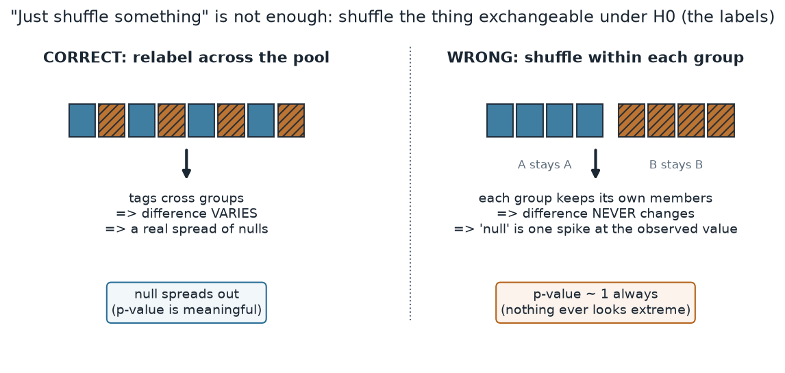
What to notice. The correct shuffle and the wrong shuffle both “shuffle something,” and both run without error — that is exactly why the mistake is easy to make. The tell is in the null distribution it produces: a correct permutation gives a spread of differences to compare against; a within-group shuffle gives no spread at all. If your permutation null has essentially no width, you have almost certainly permuted the wrong thing.

Right vs wrong shuffle (nonvisual equivalent).

Shuffle	What it breaks	Null distribution	p-value
Relabel across the pool (correct)	the label–value tie	spreads out (SD ≈ 4 points)	0.046
Shuffle within each group (wrong)	nothing that matters	a single spike at 8.62	≈ 1

Check your understanding (ungraded)

1. State the null hypothesis of this test as a claim about the label, not about the means. Why does that phrasing make “shuffle the labels” the natural thing to do?
2. The permutation null was centered at 0, but the observed difference was 8.62. Explain, in terms of exchangeability, why the null is centered at zero regardless of how far apart the two groups look.
3. The two-sided p-value was 457/10,000 ≈ 0.046. Describe in one sentence exactly what the number 457 counts.
4. A classmate reports a permutation p-value of essentially 1.0 and concludes the groups are identical. What single diagnostic would you check first, and what mistake are you looking for?

Reading guide

• Introduction to Modern Statistics (IMS) — Hypothesis testing with randomization — the closest conceptual companion to this week’s relabeling logic; read it for a second voice on why the shuffle builds the null, then check it against the figures above.
• A ModernDive — Hypothesis testing — a hands-on companion that carries out permutation tests with the infer verbs; useful for seeing the same steps expressed as code (cited, not reproduced).
• OpenIntro Statistics 4e — Inference for comparing two independent means (randomization) — reinforces the two-group setup and the two-sided tail reading.
• Learning Statistics with R (Navarro) — Hypothesis testing — a foundational-logic reference for what a p-value is and is not, independent of any particular test.

Accessibility notes

Mathematics is live text ($D_\text{obs} = \bar{x}_B - \bar{x}_A$ and $\binom{16}{8}$ render as MathML, not images). Every figure carries an alt line stating its message, an adjacent “what to notice” reading, and a data-summary table, so each point survives without the picture. Groups and shuffles are distinguished by fill, hatch, and A/B text tags (Section A solid, Section B hatched), and the null tails by hatch plus a boxed p-value label, never by color alone. A clean lint and a clean render are evidence, not a substitute for the human assistive-technology review.

Assessment (descriptive only)

This week contributes learning evidence toward building a permutation null by relabeling and reading a two-sided permutation p-value as a tail proportion. That is the shape only; the actual graded prompts, weights, and due dates live in Blackboard.

Public vs. graded. These are public, ungraded notes and practice. Graded prompts, keys, rubrics, weights, and due dates live in Blackboard Ultra, which governs.

Looking ahead

Next week we keep the shuffle but change the justification: in a randomized experiment, the relabeling is not a hypothetical about exchangeable populations — it re-enacts the coin flips that actually assigned the treatment. Same mechanics, a different and in some ways stronger warrant, and the first careful look at what a p-value does not say.