Week 6 — Bootstrap confidence intervals

Turning a bootstrap distribution into an interval — and reading what it claims

Source basis. Original instructor-authored notes; data is synthetic (40 “household incomes”, in thousands of dollars, drawn from a fixed generator, seed 45206). Open texts are conceptual companions cited by section title only (map-don’t-mine); no prose, figures, examples, or exercises are reproduced. See Open readings & attribution. Ungraded — Blackboard is authoritative for graded work.

This week. Last week you built a bootstrap distribution and read its spread. This week we take the natural next step: turn that distribution into a confidence interval by reading off its tails — the percentile interval. Then we ask the two questions that actually matter: how does it compare with the textbook $\bar{x} \pm t\,\text{SE}$ interval, and what does a 95% interval really claim?

Learning goals

By the end of this week you should be able to:

• Construct a percentile confidence interval as the middle 95% of a bootstrap distribution (here, of the sample mean).
• Compare the percentile interval with the normal/t interval $\bar{x} \pm t\cdot\text{SE}$ and say why they differ on skewed data.
• State coverage as a repeated-sampling property of the procedure — and read it off a picture of many intervals.
• Name the misreading “95% chance the parameter is in this interval,” and describe when percentile intervals undercover (small $n$, strong skew).

Where we are

We keep asking the same question: what is fragile here, and what can we still say? A single sample mean is fragile — draw another sample and it moves. Week 5 measured that movement with a bootstrap distribution. A confidence interval packages the movement into a stated range, so that instead of reporting “the mean is 51.6” we report “the mean is somewhere in a defensible interval, at a stated confidence level.”

Our running example is a batch of 40 synthetic household incomes (thousands of dollars), right-skewed. Because the data is skewed, the mean is pulled above the median — but this week the mean is exactly the quantity we want an interval for, so we bootstrap it directly.

Reading the interval off the bootstrap distribution

The percentile interval is almost embarrassingly simple: build the bootstrap distribution of the statistic, then take the 2.5th and 97.5th percentiles of those bootstrap values. Everything between them is the interval. No formula, no normal table, no assumption that the statistic is Normally distributed — the bootstrap distribution supplies its own shape.

A five-box left-to-right flow: one sample of 40 values; resample and recompute the mean B=4000 times; sort the 4000 bootstrap means; read off the 2.5th and 97.5th percentiles; the percentile interval [41.2, 63.2].

Figure 1: Building a percentile interval: resample and recompute the mean 4000 times, sort the results, and read off the 2.5th and 97.5th percentiles — here $[41.2,\ 63.2]$.

What to notice. The interval is nothing more than the middle 95% of the sorted bootstrap means. The pipeline never assumes a distribution shape; it reads the shape the resamples produce. That is the whole appeal of the percentile method.

The construction, as steps (nonvisual equivalent).

Step	What happens
1	Start with the one observed sample, $x_1,\dots,x_{40}$
2	Resample with replacement and recompute the mean, $B = 4000$ times
3	Sort the 4000 bootstrap means
4	Read off the 2.5th and 97.5th percentiles → $[41.2,\ 63.2]$

Worked example — the percentile interval

Running the bootstrap gives 4000 recomputed means. The observed mean is 51.6; the shaded middle 95% of the bootstrap means is the percentile interval.

Histogram of 4000 bootstrap means centered near 51.6 thousand dollars; a shaded band marks the middle 95 percent from 41.2 to 63.2, with dotted lines at the 2.5th percentile (41.2) and 97.5th percentile (63.2) and a solid line at the observed mean 51.6.

Figure 2: Bootstrap distribution of the mean ($B = 4000$); the shaded band is the percentile interval $[41.2,\ 63.2]$, with the observed mean at 51.6.

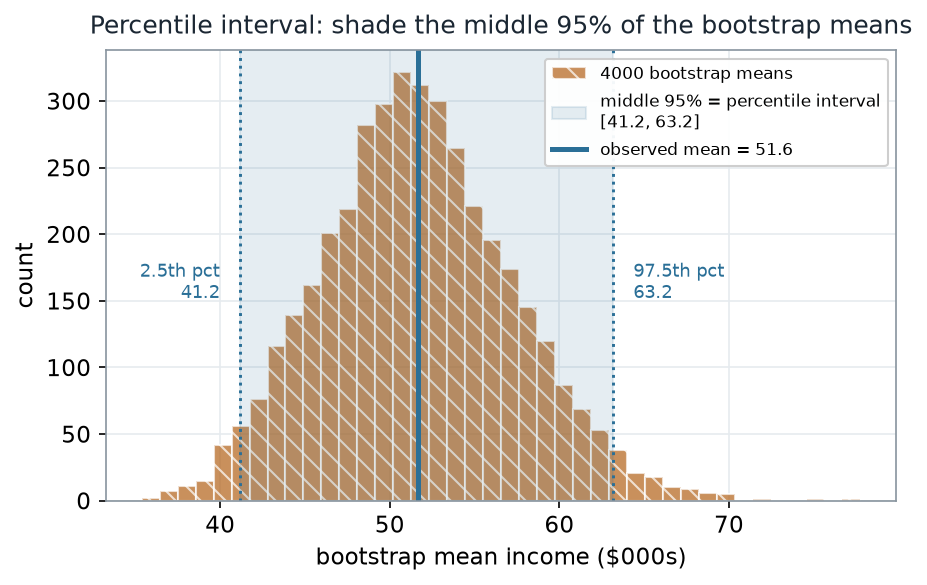
What to notice. The band is the middle 95% of the bootstrap means — 2.5% of the resampled means fall below 41.2 and 2.5% above 63.2. The interval is not centered by a formula; its edges are just two percentiles of a lightly right-skewed pile, so the upper arm (11.5) is a touch longer than the lower arm (10.5).

Percentile read-out (nonvisual equivalent).

Quantity	Value
Observed mean	51.6 ($000s) | | Bootstrap SE of the mean | 5.62 | | Percentile interval (2.5th, 97.5th) | [41.2, 63.2] | | Lower arm · upper arm (about the mean) | 10.5 · 11.5 | | Resamples ($B$)

The R you would run is short — and, as always, it contains no plotting; the picture is downstream:

# Schematic: the named data objects are the sample(s) described in the text above; this illustrates the analysis, not a self-contained runnable block.
# percentile interval for the MEAN of a skewed sample
set.seed(45206)
x    <- income                       # the 40 observed incomes ($000s)
B    <- 4000
boot <- replicate(B, mean(sample(x, size = length(x), replace = TRUE)))

quantile(boot, c(0.025, 0.975))      # the percentile interval
sd(boot)                             # bootstrap standard error of the mean

Percentile vs the t interval

The textbook interval is $\bar{x} \pm t_{0.975,\,n-1}\cdot\text{SE}$, with $\text{SE} = s/\sqrt{n}$. It is symmetric by construction: the same distance left and right of $\bar{x}$. The percentile interval is free to be asymmetric. On skewed data the two therefore disagree — subtly here, but in a way that matters as skew grows.

The bootstrap distribution of the mean drawn faintly, with two horizontal interval bars: a solid teal t interval from 40.0 to 63.3, symmetric about the mean, and a dashed ochre percentile interval from 41.2 to 63.2 with uneven arms 10.5 and 11.5.

Figure 3: The same skewed data, two intervals: the $t$ interval $[40.0,\ 63.3]$ (symmetric, $\pm 11.7$) and the percentile interval $[41.2,\ 63.2]$ (asymmetric arms $10.5 / 11.5$).

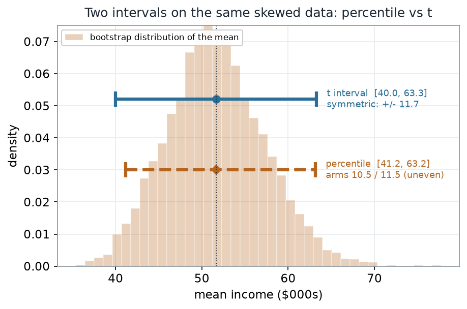
What to notice. The $t$ interval reaches down to 40.0 because it is forced to be symmetric — it spends the same 11.7 on each side of $\bar{x}$. The percentile interval only reaches 41.2 on the low side, because the bootstrap means don’t extend as far left as a symmetric rule assumes. The percentile method lets the data’s shape set the shape of the interval; the $t$ method imposes a symmetric one.

Two intervals side by side (nonvisual equivalent).

Interval	Lower	Upper	Half-width / arms	Symmetric?
$t$: $\bar{x} \pm t\cdot\text{SE}$ ($t_{0.975,39}=2.0227$)	40.0	63.3	$\pm 11.7$	yes
Percentile (2.5th, 97.5th)	41.2	63.2	10.5 / 11.5	no

What “95% confidence” actually means

Here is the honest question: what does “95%” attach to? Because our data is synthetic, we know the true mean is exactly 50, so we can do the one experiment you can never do in practice — repeat the whole study many times and watch the intervals.

Thirty horizontal percentile intervals stacked vertically, each from a fresh simulated sample, with a vertical line at the true mean 50; twenty-six intervals cross the line (solid, capture) and four miss it (dashed with an x marker).

Figure 4: Coverage as a property of the procedure: 30 repeats of the whole study. Here 26 of 30 intervals capture the true mean (50); across 1000 repeats, 92.6% capture.

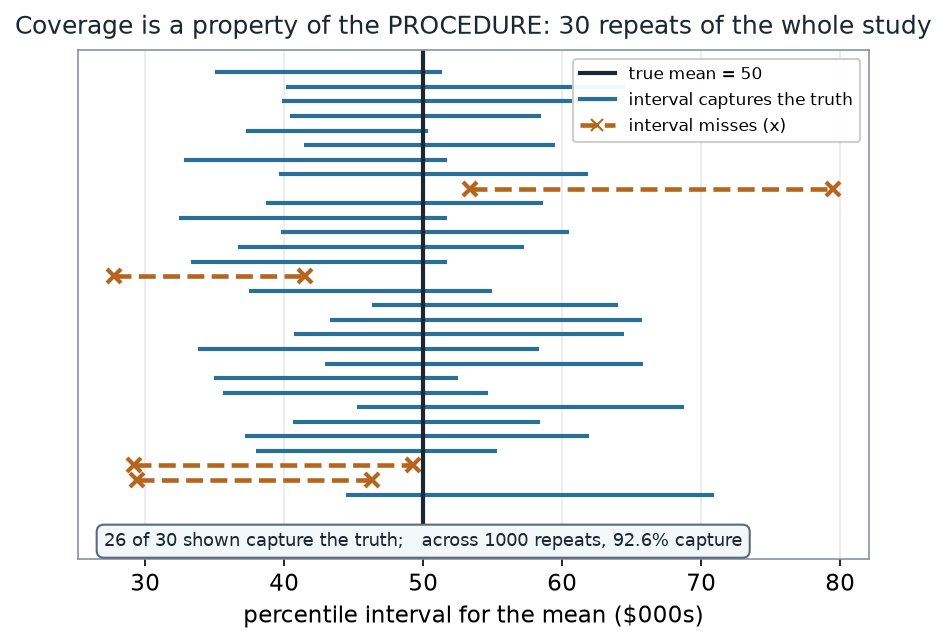
What to notice. Each repeat produces a different interval, because each starts from a different sample. “95% confidence” is a promise about the long-run share of intervals that capture the truth, not about any single one. Read that share off the many intervals — it is a property of the recipe, seen only by repeating the recipe.

Coverage read-out (nonvisual equivalent).

Quantity	Value
True mean (known, synthetic)	50 ($000s)
Repeats simulated	1000
Intervals capturing the truth	92.6%
Shown in the figure	26 of 30 capture

A common mistake

“A 95% interval means there’s a 95% chance the mean is in this interval.” Once you have a particular interval, the mean is either inside it or not — the probability is 0 or 1, we just don’t know which. The 95% describes how often the procedure captures the truth across many samples, not the odds for your one interval. And the promise is not automatic: for the mean of skewed data with small $n$, the percentile interval undercovers — here it captured only 92.6% of the time, short of the nominal 95%.

Twenty-five percentile intervals against a fixed vertical line at the true mean 50; two intervals miss the line and are highlighted in dashed ochre with x markers, while one interval labeled THIS study’s interval is drawn in bold at the top; a caption notes the 95% is the long-run capture rate of the procedure.

Figure 5: The misread, pictured: the truth (50) is fixed; each interval either contains it or not. Of these 25 intervals, 2 miss. “THIS study’s interval” is just one draw — the 95% is the procedure’s capture rate, not a probability for it.

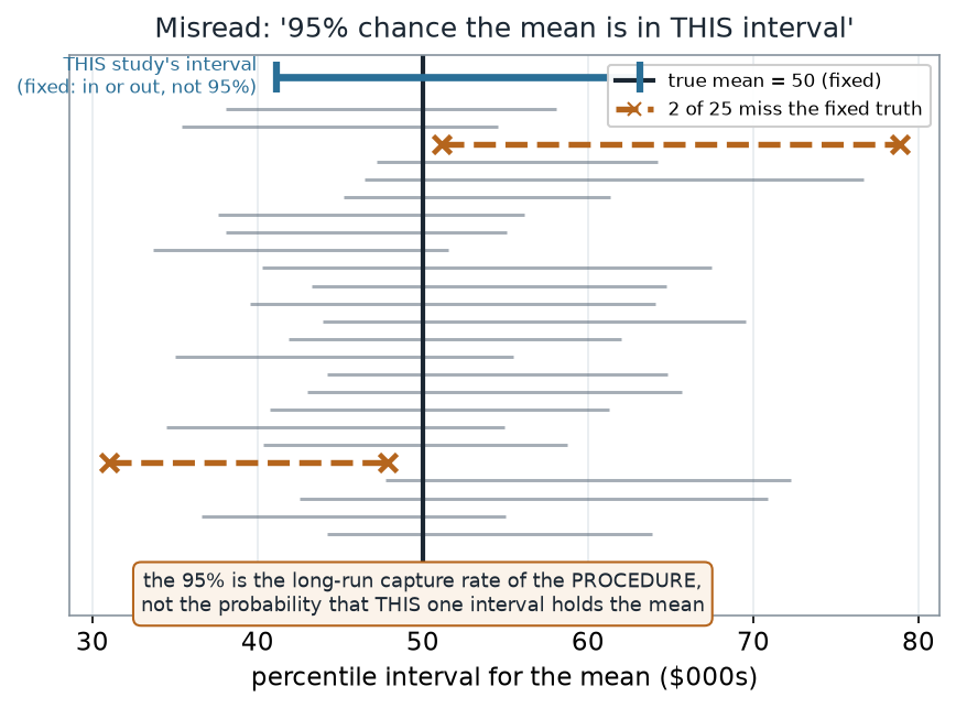
What to notice. The vertical truth line does not move; the intervals do. Highlighting the misses makes the point concrete: you cannot assign “95%” to the single bold interval at the top, because it is fixed. The confidence level lives in the collection, not the individual.

Misread read-out (nonvisual equivalent).

Quantity	Value
Intervals shown	25
Intervals missing the fixed truth	2
Probability the truth is in a given fixed interval	0 or 1 (unknown)

Check your understanding (ungraded)

1. In one sentence, describe how to build a percentile interval from a bootstrap distribution — what two numbers do you read off, and from what?
2. The $t$ interval here was $[40.0, 63.3]$ and the percentile interval was $[41.2, 63.2]$. Explain why the low ends differ, in terms of the shape of the bootstrap distribution.
3. A classmate says “the 95% interval $[41.2, 63.2]$ has a 95% chance of containing the mean.” Rewrite the claim so it is correct.
4. Coverage came out 92.6%, below the nominal 95%. Name the two features of this problem that push the percentile interval to undercover, and say what you might do about it.

Reading guide

• IMS — Bootstrap confidence intervals — a conceptual companion to reading an interval off a bootstrap distribution; read for the intuition, then check it against the pictures above.
• ModernDive — Bootstrapping and confidence intervals — reinforces the percentile method and the repeated-sampling meaning of a confidence level.
• OpenIntro Statistics 4e — Confidence intervals — the $\bar{x}\pm t\cdot\text{SE}$ interval we contrast against, for a common reference point.
• NIST/SEMATECH e-Handbook — Bootstrap uncertainty — an instructor reference on bootstrap interval methods and their limits (cited, not reproduced).

Accessibility notes

Mathematics is live text ($\bar{x} \pm t\cdot\text{SE}$ renders as MathML, not an image). Every figure carries an alt line stating its message, a “what to notice” reading, and an adjacent data-summary table, so each point survives without the picture. Intervals are distinguished by linestyle and marker (solid = the $t$ interval / a capturing interval; dashed with an “×” = the percentile interval / a missing interval) and by labels, not color alone. A clean lint and a clean render are evidence; the rendered assistive-technology review is a human step.

Assessment (descriptive only)

This week contributes learning evidence toward constructing and reading a percentile confidence interval and stating what a confidence level claims. That is the shape only; the actual graded prompts, weightings, and due dates live in Blackboard.

Public vs. graded. These are public, ungraded notes and practice. Graded prompts, keys, rubrics, weightings, and due dates live in Blackboard Ultra, which governs.

Looking ahead

We now have two ways to make an interval — a formula and a resample — and a clear-eyed view of what either one claims. Next week we leave the mean behind and return to ranks, building distribution-free procedures for one-sample and paired data where even the bootstrap’s assumptions are more than we want to make.