Week 8 — Two-sample rank methods

Wilcoxon rank-sum, Mann–Whitney, and what a rank test really compares

Source basis. Original instructor-authored notes; data is synthetic (two groups of “recovery times” in days, drawn from a fixed generator, seed 45208). Open texts are conceptual companions cited by section title only (map-don’t-mine); no prose, figures, examples, or exercises are reproduced. See Open readings & attribution. Ungraded — Blackboard is authoritative for graded work.

This week. Last week we ranked within-pair differences for matched data. Now the two groups are independent — different patients under two care plans — so there is no pairing to lean on. The move is the same rank idea scaled up: pool both groups, rank everything together, and ask whether one group’s ranks run systematically high. That is the Wilcoxon rank-sum test, and its twin the Mann–Whitney U. The null is the permutation null you already met in Weeks 3–4.

Learning goals

By the end of this week you should be able to:

• Pool and rank two independent samples and compute the rank-sum $W$ of one group.
• Convert between the rank-sum $W$ and the Mann–Whitney $U$, and read $U/(n_1 n_2)$ as an estimate of $P(A > B)$.
• Build the permutation null of the rank-sum by shuffling group labels, and read a two-sided p-value from it.
• State the location-shift interpretation — and the caveat that when the two shapes differ, the rank-sum tests stochastic dominance, not a difference in means.

Where we are

Two care plans, two independent groups of recovery times (days): standard care ($n_1 = 10$) and a new protocol ($n_2 = 12$). The samples are small and right-skewed, with a long recovery in each group — exactly the setting where a mean-and-t comparison is fragile and a rank method earns its keep. A rank test throws away the raw distances and keeps only the ordering, which is why one stray long recovery cannot drag the conclusion around.

The whole test starts with one move: pool all $n_1 + n_2 = 22$ values and rank them together, from 1 (fastest recovery) to 22 (slowest), averaging any ties. The rank-sum of the standard-care group — just add up the ranks its ten patients received — is the test statistic.

A rank axis from 1 to 22. Standard-care observations (filled circles, top row) sit almost entirely at ranks 10 and above; new-protocol observations (open squares, bottom row) fill the low ranks 1 through 9 with three exceptions at ranks 17, 18, and 22. A box reads: rank-sum of standard care W = 151 of 253 total ranks.

Figure 1: Pool both groups and rank all 22 recovery times. The standard-care ranks pile up at the high end; their rank-sum is $W = 151$ out of $253$ total ranks.

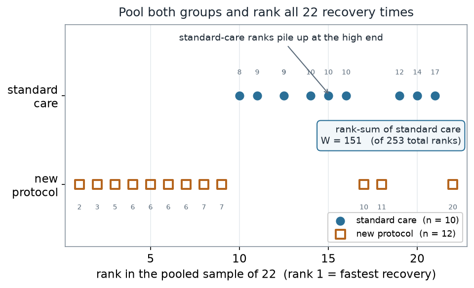
What to notice. Notice the standard-care circles cluster at the high ranks (slow recoveries) while the new-protocol squares hold the low ranks (fast recoveries). If the two plans were interchangeable, each group would collect a fair share of high and low ranks; instead standard care collected $W = 151$ of the $253$ total ranks. The question the test answers is whether $151$ is surprisingly high.

The two groups, as numbers (nonvisual equivalent).

Group	$n$	median (days)	rank-sum $W$	Mann–Whitney $U$
Standard care (A)	10	9.8	151	96
New protocol (B)	12	6.0	102	24
Pooled total	22	—	253	120

The rank-sum test, step by step

The rank-sum $W$ is only half the picture; we need a reference distribution to judge it against. Under the null hypothesis that the two plans are exchangeable — a patient’s recovery would have been the same under either label — the group labels carry no information. So we can shuffle the labels across the fixed set of ranks, recompute the rank-sum each time, and see how far out $W = 151$ falls.

A five-box vertical flow diagram. Box 1: pool both groups into one set of 22 values. Box 2: rank all 22 values 1 to 22, averaging ties. Box 3: add up one group’s ranks to get W for standard care. Box 4: shuffle the group labels many times to build a null distribution of W. Box 5: the p-value is the share of shuffles whose W is at least as far from the center as the observed W. A footnote reads observed W = 151, p = 0.016.

Figure 2: The Wilcoxon rank-sum / Mann–Whitney procedure: pool, rank, sum one group’s ranks, then judge that sum against a null built by shuffling the labels.

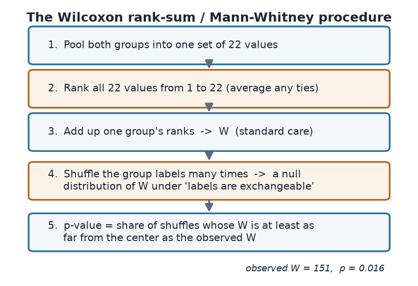
What to notice. Every step is distribution-free: nothing here assumes normal data. The only quantities that move are the labels; the pooled ranks stay fixed, so — when there are no ties — the null distribution of $W$ depends only on the sample sizes, not on the shape of the data. Ties leave a faint mark (the two $9.4$-day recoveries share the average rank $12.5$, so the rank multiset carries a small correction the exact permutation already folds in), but the appeal of a rank method stands: the data’s shape barely touches the null.

The procedure, as steps (nonvisual equivalent).

Step	What you do	Result here
1	Pool the 22 values	one combined sample
2	Rank 1–22, averaging ties	ranks fixed
3	Sum the standard-care ranks	$W = 151$
4	Shuffle labels many times	null of $W$
5	Compare $W$ to the null	two-sided $p = 0.016$

The R you would run is short, and — as always — it contains no plotting; the picture is downstream:

# two independent groups of recovery times (days)
standard <- c(7.5, 9.2, 9.4, 9.4, 9.7, 9.8, 10.2, 11.5, 14.5, 17.0)   # n = 10
newprot  <- c(2.0, 3.3, 4.9, 5.6, 5.7, 5.9, 6.0, 6.7, 7.0, 10.4, 11.4, 20.0)  # n = 12

# pool, rank (average ties), and sum the standard-care ranks
r <- rank(c(standard, newprot))
W <- sum(head(r, length(standard)))         # rank-sum of standard care = 151

# Mann-Whitney U (R's wilcox.test reports U, labelled "W" in its output)
U <- W - length(standard) * (length(standard) + 1) / 2   # 96
wilcox.test(standard, newprot)              # two-sample rank-sum / Mann-Whitney

# a permutation null of the rank-sum: shuffle the labels across the fixed ranks
set.seed(45208)
B      <- 50000
centre <- mean(r) * length(standard)        # null mean of W = 115
Wnull  <- replicate(B, sum(sample(r, length(standard))))
mean(abs(Wnull - centre) >= abs(W - centre))   # two-sided permutation p-value

Worked example — a rank-sum test of recovery times

Run the shuffle 50,000 times and the null distribution of $W$ takes shape. Its center is $\mu_W = n_1(N+1)/2 = 10 \times 23 / 2 = 115$; the observed rank-sum sits well out in the upper tail.

A histogram of the permutation null distribution of the rank-sum W, roughly bell-shaped and centered at 115. A dotted line marks the null center 115; a solid line marks the observed W = 151 far to the right. The two tails beyond 36 units from the center are hatched, labeled two-sided p = 0.016.

Figure 3: Permutation null of the rank-sum from 50,000 label shuffles, centered at $115$. The observed $W = 151$ lies $36$ ranks out; the shaded two tails give a two-sided $p = 0.016$.

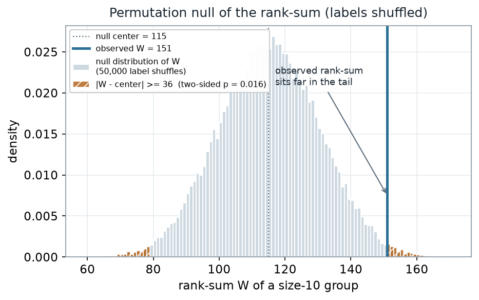
What to notice. The observed rank-sum is $36$ ranks above the null center — about $2.4$ null standard deviations ($36 / 15.13$). Only about $1.6\%$ of label shuffles land a rank-sum that far from the center in either direction, so the two-sided permutation p-value is $0.016$. (We use the $(1 + \text{count})/(1 + B)$ convention, which never reports a p of exactly zero.) The evidence says the two plans are not interchangeable: standard-care recoveries run systematically slower.

Rank-sum read-out (nonvisual equivalent).

Quantity	Value
Observed rank-sum $W$ (standard care)	151
Null center $\mu_W = n_1(N+1)/2$	115
Null SD of $W$	15.13
Mann–Whitney $U = W - n_1(n_1{+}1)/2$	96
$U/(n_1 n_2)$ = estimate of $P(A > B)$	0.80
Two-sided permutation p (B = 50,000)	0.016

The Mann–Whitney $U = 96$ carries a plain-language reading. Of the $n_1 n_2 = 120$ possible patient-to-patient matchups (one standard, one new), the standard-care patient recovered slower in $96$ of them — so $U/(n_1 n_2) = 0.80$ estimates $P(\text{standard} > \text{new})$. Rank-sum and $U$ are the same test: $U$ is just $W$ with the group’s minimum possible rank-sum, $n_1(n_1{+}1)/2 = 55$, subtracted off.

What a significant rank-sum does (and does not) say

A small p tells you the groups differ, but differ how? The cleanest interpretation holds when the two distributions have the same shape and differ only by a horizontal shift — the location-shift model. Under that model the rank-sum tests whether the shift is zero, and the shift has a natural estimate: the Hodges–Lehmann estimator, the median of all $n_1 n_2$ pairwise differences, which here is $3.8$ days.

Two right-skewed density curves of identical shape. A solid teal curve (new protocol) peaks near 6 days; a dashed ochre curve (standard care) is the same curve slid 3 days to the right. Dotted vertical lines mark the two medians, and a double-headed arrow between them is labeled shift = 3 days — the population model shift; the sample estimate given in the caption is 3.8 days.

Figure 4: The location-shift model: two distributions of identical shape, one slid to the right by a fixed amount. The picture shows the population model — a clean 3-day shift between the two curves; on our sample, the rank-sum’s estimated shift (the difference in medians, and the Hodges–Lehmann estimator) is $3.8$ days.

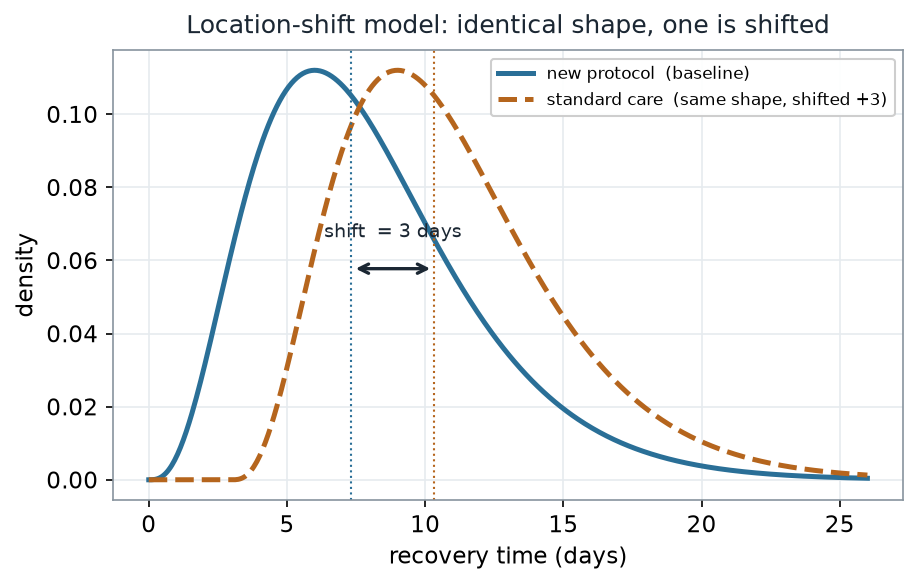
What to notice. The curves are drawn from the population model — a clean $3$-day shift between two identical shapes — and the sample lands right beside it. When the shapes match, “standard care runs about $3.8$ days slower” is a fair, compact summary, and the difference in sample medians ($9.8 - 6.0 = 3.8$ days) agrees with the Hodges–Lehmann estimate. The rank test earns this reading because the only difference between the curves is where they sit, not how they are shaped.

Shift read-out (nonvisual equivalent).

Quantity	Value
Median, new protocol	6.0 days
Median, standard care	9.8 days
Difference in sample medians	3.8 days
Hodges–Lehmann shift estimate	3.8 days
$P(\text{standard} > \text{new})$ estimate	0.80

A common mistake

“A significant rank-sum means the means differ, so it’s just a robust t-test.” It is not. The rank-sum compares whole distributions through $P(A > B)$ — the tendency of one group to outrank the other — not $\mu_A - \mu_B$. Reading the result as a clean difference in centers is only safe under the location-shift model, where the two shapes are the same. When the shapes differ, a significant rank-sum signals stochastic dominance (one group tends to produce larger values), and “difference in means” can be flatly wrong — even zero.

When the two shapes differ

Here is the caveat made concrete. Two groups can share the exact same mean yet be so differently shaped that the rank-sum still leans hard toward one of them.

Two density curves with the same mean of 10, marked by a dotted vertical line at 10. A solid teal curve (group X) is symmetric with median 10. A dashed ochre curve (group Y) is strongly right-skewed with its bulk below 10 (median 8.3) and a long upper tail. An annotation reads: equal means, unequal shapes; the rank-sum reflects P(Y > X) = 0.40, not the difference in means (which is 0).

Figure 5: Two groups with the same mean ($10$ days) but different shapes: symmetric (median $10$) versus right-skewed (median $8.3$). The rank-sum sees $P(Y > X) = 0.40$, not the zero difference in means.

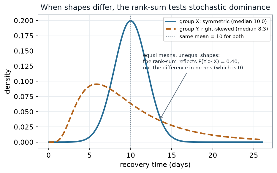
What to notice. Both groups average $10$ days, so a t-test targets a difference of zero. But the skewed group $Y$ spends most of its mass below $10$ (its median is $8.3$), pulled up to a mean of $10$ only by a long upper tail. A randomly chosen $Y$ beats a randomly chosen $X$ only $40\%$ of the time, so the rank-sum leans toward $X$. The two tests are answering different questions — the rank-sum is a test about $P(Y > X)$, not about the means.

Shape-difference read-out (nonvisual equivalent).

Distribution	Mean	Median	$P(Y > X)$
Group X (symmetric)	10.0	10.0	—
Group Y (right-skewed)	10.0	8.3	—
Comparison	equal	differ	0.40

Check your understanding (ungraded)

1. In your own words, why does pooling and ranking make the rank-sum’s null distribution depend only on $n_1$ and $n_2$ — when there are no ties — rather than on the shape of the data? What does a tie (like the two $9.4$-day recoveries) change?
2. The observed rank-sum was $W = 151$ with a null center of $115$. Explain what the permutation null is a distribution of, and why a rank-sum far from $115$ counts as evidence.
3. The Mann–Whitney $U = 96$ gave $U/(n_1 n_2) = 0.80$. State in a sentence what real-world quantity $0.80$ estimates.
4. Two groups have identical means but a significant rank-sum. Is that a contradiction? Explain what the rank-sum is actually detecting, and when “difference in means” would have been a safe reading.

Reading guide

• IMS — comparing two independent groups — a conceptual companion to two-group comparison; read it for the framing, then map it onto the rank-based null above.
• Learning Statistics with R (Navarro) — nonparametric alternatives to the two-sample t-test — an instructor reference on where the Mann–Whitney fits beside the t-test (cited, not reproduced).
• NIST/SEMATECH e-Handbook — two-sample rank-based location tests — reinforces the location-shift interpretation and its assumptions.

Accessibility notes

Mathematics is live text ($W = n_1(N{+}1)/2$ renders as MathML, not an image). Every figure carries an alt line stating its message, a “what to notice” reading, and an adjacent data-summary table, so each point survives without the picture. Groups are distinguished by marker and linestyle (standard care = filled circle / solid; new protocol = open square / dashed) and by labels, never by color alone. A clean lint and a clean render are evidence; the rendered assistive-technology review is a human step.

Assessment (descriptive only)

This week contributes learning evidence toward running a two-sample rank test and reading its permutation null and stating the location-shift interpretation and its limits. That is the shape only; the actual graded prompts, values, and due dates live in Blackboard.

Public vs. graded. These are public, ungraded notes and practice. Graded prompts, keys, rubrics, point values, and due dates live in Blackboard Ultra, which governs.

Looking ahead

Next week we move from ranks to counts: categorical and ordinal outcomes across two groups, where an exact (permutation) null again beats a shaky large-sample approximation when the table is small — and where treating ordered categories as interval numbers is its own tempting mistake.