Week 4 — Randomization tests

Inference from the coin the experiment actually flipped

Source basis. Original instructor-authored notes; data is synthetic (a randomized field trial of 20 plots — 10 treatment, 10 control — from a fixed generator, seed 45204). Open texts are conceptual companions cited by section title only (map-don’t-mine); no prose, figures, examples, or exercises are reproduced. See Open readings & attribution. Ungraded — Blackboard is authoritative for graded work.

This week. Last week we shuffled group labels to ask whether a difference could be an accident of which unit landed in which group. This week we take the same shuffling machinery but change the warrant: in a randomized experiment the shuffling is not a modelling assumption we hope holds — it is a physical fact of how the study was run. The randomization test asks: among all the label assignments the experiment’s own coin could have produced, how unusual is the one we got?

Learning goals

By the end of this week you should be able to:

Explain why a randomization test draws its reference distribution from the study’s actual random assignment, not from an assumed population.
Build a randomization distribution of a treatment effect by re-randomizing the labels under the sharp null of no unit-level effect.
Compute and read a two-sided randomization p-value as a shaded share of that distribution.
State precisely what that p-value does and does not claim — including that it is not the probability the null is true, and that it speaks only to the units that were randomized.

Where we are

We keep asking what is fragile here, and what can we still say? In an observational comparison, the fragile part is the leap from “these groups differ” to “the difference is real” — we never saw the coin that sorted units into groups, so we have to assume one. A randomized experiment removes that fragility at the source. The experimenter physically randomizes units to treatment or control, so the only thing separating the two groups — before any treatment acts — is the luck of the draw.

That gives inference a footing that needs no population at all. If the treatment truly did nothing, then each plot’s yield would be exactly what it is regardless of the label it received (this is the sharp null). Under that null the observed difference is manufactured entirely by which plots happened to be called “treatment.” So we can rebuild the whole space of “what could have happened” by simply re-dealing the labels — the same 20 numbers, reshuffled into two groups of ten.

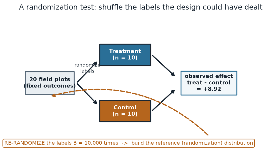
Flow diagram: a box of 20 field plots with fixed outcomes splits by randomized labels into a Treatment box (n=10) and a Control box (n=10); both feed an observed-effect box reading treatment minus control equals plus 8.92; a dashed loop arrow returns to the plots labeled re-randomize the labels 10,000 times to build the reference distribution.

What to notice. The 20 outcomes are treated as fixed; only the labels move. The observed effect (+8.92 bushels) is one draw from the label-shuffling process. The dashed loop is the whole method: re-randomize, recompute the difference, repeat — the collection of those differences is the reference distribution against which +8.92 is judged.

The experiment, as numbers (nonvisual equivalent).

Group	n	Mean yield	Sorted yields (bushels/plot)
Control	10	47.88	40.8, 41.7, 43.5, 43.6, 43.8, 47.0, 48.2, 52.5, 57.4, 60.3
Treatment	10	56.80	42.9, 49.9, 52.8, 53.9, 54.7, 59.0, 59.7, 61.9, 65.4, 67.8
Observed effect		+8.92	treatment mean − control mean

Building the randomization distribution

There are $\binom{20}{10} = 184{,}756$ ways to split 20 plots into two groups of ten — every one of them was equally likely when the experiment was randomized. Enumerating all of them is possible here but unnecessary; we approximate the reference distribution by drawing a large Monte Carlo sample of re-randomizations. Each re-randomization deals the labels afresh and recomputes the treatment-minus-control mean.

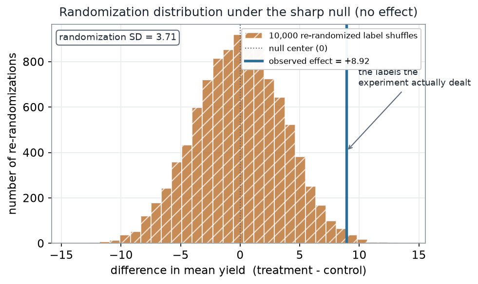
Histogram of 10,000 re-randomized treatment-minus-control mean differences, roughly bell-shaped and centered at 0 with a spread of about plus or minus 10; a solid vertical line marks the observed effect of plus 8.92 far out in the right tail, with a note that these are the labels the experiment actually dealt.

What to notice. The reference distribution is centered at 0 — under the sharp null, re-labeling should help treatment and control equally often, so the typical manufactured difference is nothing. Its spread (SD ≈ 3.71) is the natural sampling-to-sampling wobble of the label lottery. The observed +8.92 is more than two of those SDs out; almost none of the reshuffles reach it.

The reference distribution, as numbers.

Quantity	Value
Re-randomizations (B)	10,000
Center (null)	0
Randomization SD (spread)	3.71
Range of re-randomized differences	−13.9 to +13.6
Observed effect	+8.92

The R you would run is short — and notice there is no plotting in it; the picture is downstream:

# Schematic: the named data objects are the sample(s) described in the text above; this illustrates the analysis, not a self-contained runnable block.
# design-based randomization test: re-deal the labels the experiment could have produced
set.seed(45204)
yield <- c(treatment, control)          # the 20 FIXED outcomes under the sharp null
label <- rep(c("T", "C"), each = 10)    # the assignment that actually happened
obs   <- mean(yield[label == "T"]) - mean(yield[label == "C"])

B     <- 10000
diffs <- replicate(B, {
  shuffled <- sample(label)             # one label assignment the design could have dealt
  mean(yield[shuffled == "T"]) - mean(yield[shuffled == "C"])
})

sd(diffs)                                       # spread of the randomization distribution
(1 + sum(abs(diffs) >= abs(obs))) / (1 + B)     # two-sided p-value, +1 convention

Worked example — the two-sided p-value

We had no prior reason to bet on treatment helping rather than hurting, so we ask a two-sided question: how often does re-randomization alone produce a difference at least as far from zero as our +8.92, in either direction? That share is the two-sided randomization p-value.

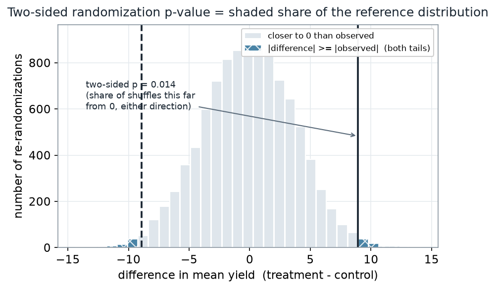
The same randomization histogram with both tails shaded where the absolute difference is at least 8.92; solid and dashed vertical lines mark plus and minus 8.92; an annotation reads two-sided p equals 0.014, the share of shuffles this far from zero in either direction.

What to notice. Both tails are shaded — a difference of −8.92 would have been just as surprising as +8.92. Out of 10,000 reshuffles, only 135 were that extreme, so with the +1 convention $p = (1 + 135)/(1 + 10{,}000) = 0.014$ . Reading it plainly: if the treatment did nothing, a gap this large would arise from label luck about 1.4% of the time. The one-sided version (treatment ≥ control) is smaller still, $p = 0.007$ .

Two-sided p-value read-out (nonvisual equivalent).

Quantity	Value
Observed effect	+8.92 bushels
Re-randomizations at least as extreme (both tails)	135 of 10,000
Two-sided p-value (+1 convention)	0.014
One-sided p-value (treatment ≥ control)	0.007

The +1 convention — adding one to both the count and the denominator — counts the actually-observed assignment as one of the possibilities (it is always as extreme as itself). It keeps the p-value from ever being exactly zero, which matters because a Monte Carlo run of 10,000 shuffles is only an estimate.

Permutation last week, randomization this week

The arithmetic this week is identical to last week’s permutation test — shuffle labels, recompute, count the tail. What changes is the story that licenses the conclusion. A permutation test imagines an exchangeable population and asks whether the labels could be swapped without changing the distribution. A randomization test needs no population: the reference distribution is generated by the physical act of randomization the experimenter performed, so the inference is design-based.

Permutation logic (a population and exchangeability) versus randomization logic (the design that was actually run): same arithmetic, different warrant for the inference.

Aspect	Permutation test (Week 3)	Randomization test (this week)
Where the randomness lives	An assumed exchangeable population	The experiment’s own random assignment
Null hypothesis	The two groups share one distribution	Sharp null: no unit gets a different outcome from its label
What is held fixed	The pooled values	The 20 outcomes (potential outcomes under the null)
Warrant for inference	A modelling assumption (exchangeability)	A physical fact (units were randomized)
Inference generalizes to	The assumed population	The units that were randomized

What to notice. The two columns run the same shuffle, so their p-values often coincide — but their warrant differs. Randomization inference is the sturdier of the two precisely because its “if the null were true, here is what could have happened” is not a hope about a population; it is a rerun of the coin the experimenter actually flipped.

A common mistake

“p = 0.014, so there’s a 1.4% chance the treatment does nothing.” No. The p-value is computed assuming the null is true and reports how often chance re-labeling would manufacture an effect this large — it is $P(\text{data this extreme} \mid \text{null})$ , not $P(\text{null} \mid \text{data})$ . Two more traps travel with it: a small p-value does not mean the effect is large (the effect’s size is +8.92 bushels; the p-value only says it is surprising), and a randomization result generalizes only to the units actually randomized — these 20 plots — not automatically to every field, crop, or season.

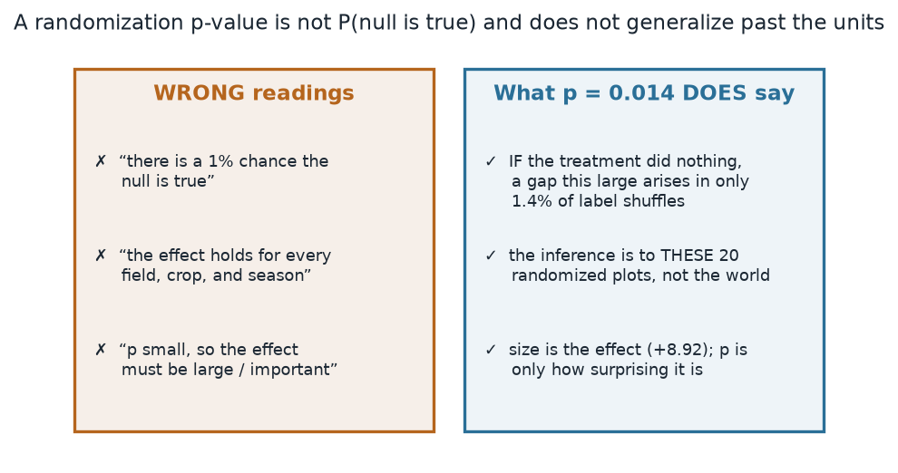
Two-column diagram. Left, labeled WRONG readings, lists three crossed-out claims: a 1% chance the null is true, the effect holds for every field crop and season, and p small so the effect must be large. Right, labeled what p equals 0.014 does say, lists three checked claims: if the treatment did nothing a gap this large arises in only 1.4% of shuffles, the inference is to these 20 randomized plots not the world, and size is the effect plus 8.92 while p is only how surprising it is.

What to notice. Keep the effect and the p-value as two separate facts. The effect is how big (+8.92 bushels); the p-value is how surprising it would be under the null (0.014). A responsible sentence reports both, and names the population it applies to.

The three misreadings, corrected (nonvisual equivalent).

Wrong reading	What is actually true
“1.4% chance the null is true”	If the null were true, chance labeling gives an effect this big 1.4% of the time
“Holds for every field and season”	Applies to the 20 randomized plots; broader claims need broader randomization
“Small p ⇒ large/important effect”	Size is the effect (+8.92); p only measures surprise

Check your understanding (ungraded)

In a randomization test, what exactly is held fixed across all the re-randomizations, and what is allowed to vary? Why does that split match how the experiment was actually run?
The randomization distribution was centered at 0. Explain in one sentence why 0 is its natural center under the sharp null.
Our two-sided p-value was 0.014 and the one-sided was 0.007. Why is the two-sided value roughly twice the one-sided one here, and when would you report each?
A colleague concludes, “p = 0.014, so this fertilizer will raise yields on any farm.” Name two things wrong with that sentence, using this week’s vocabulary.

Reading guide

IMS — Randomization and inference for a difference — a conceptual companion to shuffling labels to test a difference; read for the intuition, then check it against the reference distribution above.
OpenIntro Statistics 4e — inference for comparing two means (randomization) — reinforces the two-group comparison and the tail-area reading of a p-value.
NIST/SEMATECH e-Handbook — Randomization in the design of experiments — an instructor reference on why physical randomization is what licenses design-based inference (cited, not reproduced).

Accessibility notes

Mathematics is live text ( $\binom{20}{10}$ and $P(\text{data}\mid\text{null})$ render as MathML, not an image). Every figure carries an alt line stating its message, a “what to notice” reading, and an adjacent data-summary table, so each point survives without the picture. The figures are distinguished by linestyle and hatch, never by color alone: in the randomization distribution the observed effect is a solid teal line and the re-randomized shuffles are an ochre-hatched histogram; in the p-value figure the observed effect and its mirror bound are solid and dashed ink lines while the two extreme tails are teal cross-hatched bars against plain-grey central bars. A clean lint and a clean render are evidence; the rendered assistive-technology review is a human step.

Assessment (descriptive only)

This week contributes learning evidence toward building a randomization distribution by re-randomizing labels and stating precisely what a randomization p-value claims. That is the shape only; the actual graded prompts, points, and due dates live in Blackboard.

Public vs. graded. These are public, ungraded notes and practice. Graded prompts, keys, rubrics, point values, and due dates live in Blackboard Ultra, which governs.

Looking ahead

Next week we stop testing a difference and start estimating one. The bootstrap reuses the resampling instinct — but instead of shuffling labels under a null, it resamples the data itself to ask how much a summary would wobble from sample to sample, and turns that wobble into a confidence interval.