Week 1 — Statistical decisions, actions, loss, and risk
Where this week starts
Week 0 closed with two estimators of a success probability whose risk curves crossed, and left that comparison deliberately unresolved. This week it becomes the subject. Every procedure the course studies afterwards — a test, a confidence set, a shrinkage estimator, a robust M-estimator, a posterior decision — is a rule turning data into an action, and every claim about such a rule concerns its behaviour averaged over data you have not yet seen. The vocabulary is short: an estimand, an action space, a loss function, a procedure, and a risk function.
What the previous course left unfinished is the comparison step. You learned to compute the mean squared error of an estimator and to prefer the smaller value. What is rarely said is that the value is the height at one parameter point of a function defined over the whole parameter space, and two such functions usually cross. Once they cross, “smaller mean squared error” is an incomplete sentence whose missing half is either “at which \(\theta\)” or “averaged against what”. That grammar is built here, before any test appears, because a test is a decision problem whose action space has two elements.
Three things should feel different by the end. You should write risk as \(R(\theta, \delta)\) with both arguments visible, not as a single quantity attached to an estimator. You should expect most pairs of procedures to be incomparable, and treat the claim that one is simply better as needing an unusual kind of evidence. And you should notice that you choose a loss function whether or not you write one down, and that changing it changes the recommended action even when data, model, and sample size are untouched.
Why this matters beyond the theorem
A laboratory chooses between two ways of estimating a mean concentration and settles the question with a simulation run at one plausible value of the true mean. The shrunken estimator wins on mean squared error, is adopted, and is then applied for two years to specimens whose concentrations are nothing like the simulated one. Nobody was dishonest; the study established a fact about one point of a risk function and used it as a fact about the function. The first worked example below has that shape exactly: shrinkage cuts the risk by more than a third at one parameter value and more than doubles it six standard errors away.
The same gap opens on the decision side. A quality engineer sets an inspection cutoff — reject the batch if at least two of twenty-five inspected units are defective — without writing down what rejecting a good batch costs relative to accepting a bad one. The cutoff still encodes a ratio; it encodes an unexamined one. When the cost of rejection later rises the cutoff ought to move, and it will not unless someone recognizes it was a loss ratio all along.
What you will be able to do
- Write a statistical problem in decision-theoretic form: name the estimand, the action space, the loss, the procedure, and the risk, and say which of them are modelling choices rather than facts about the data.
- Derive a risk function exactly under squared-error loss from the variance-plus-squared-bias decomposition, and locate where two risk curves cross.
- State the conditions under which the optimal action is a mean, a median, or a mode of the available belief, and explain why the three differ on a skewed one.
- Decide whether one procedure dominates another, say what admissibility does and does not promise, and give an admissible procedure nobody should use.
- Compute the Bayes risk and the maximum risk of a procedure, and exhibit a pair the two summaries rank in opposite orders.
- Derive the optimal action in a two-action problem with asymmetric loss and show how its cutoff moves with the loss ratio.
Terms and notation worth fixing
Fix these now; the rest of the course uses them without re-explanation. The convention that matters most is the last one: risk carries two arguments, always.
| Symbol or term | Meaning as used in this course |
|---|---|
| estimand | the feature the decision is about: \(\theta\), a component of it, or a function \(g(\theta)\) |
| \(\mathcal{A}\) | the action space: the real line, a set of intervals, or a two-element set such as accept or reject |
| \(L(\theta, a)\) | the loss when nature is at \(\theta\) and the action is \(a\); a modelling choice, not a fact about the data |
| \(\delta\) | a procedure, a function from the sample space to \(\mathcal{A}\), so \(\delta(x)\) is the action taken when \(x\) is observed |
| \(R(\theta, \delta)\) | the risk, \(E_\theta L(\theta, \delta(X))\): loss averaged over the data at a fixed \(\theta\), hence a function on \(\Theta\) |
| domination | \(\delta_1\) dominates \(\delta_2\) when \(R(\theta, \delta_1) \le R(\theta, \delta_2)\) for all \(\theta\), strictly somewhere; \(\delta\) is admissible when nothing dominates it |
| \(r(\pi, \delta)\) | the Bayes risk \(\int_\Theta R(\theta, \delta) \, \pi(d\theta)\), the risk curve averaged against a prior |
| \(\sup_\theta R(\theta, \delta)\) | the maximum risk, the worst height on the curve; the summary a minimax rule minimizes |
The anatomy of a statistical decision
A decision problem has five parts arriving in a fixed order. Nature selects \(\theta \in \Theta\) and never reveals it. The data \(X\) arrive from \(f(x; \theta)\). A procedure \(\delta\) converts the observed \(x\) into an action \(a = \delta(x)\) in the action space \(\mathcal{A}\). The loss \(L(\theta, a)\) prices the mismatch between action and state. Because that loss involves the unobserved \(\theta\) and the random \(X\), it cannot be evaluated in practice; what can be studied is its average at each fixed parameter value, the risk \(R(\theta, \delta) = E_\theta L(\theta, \delta(X))\).
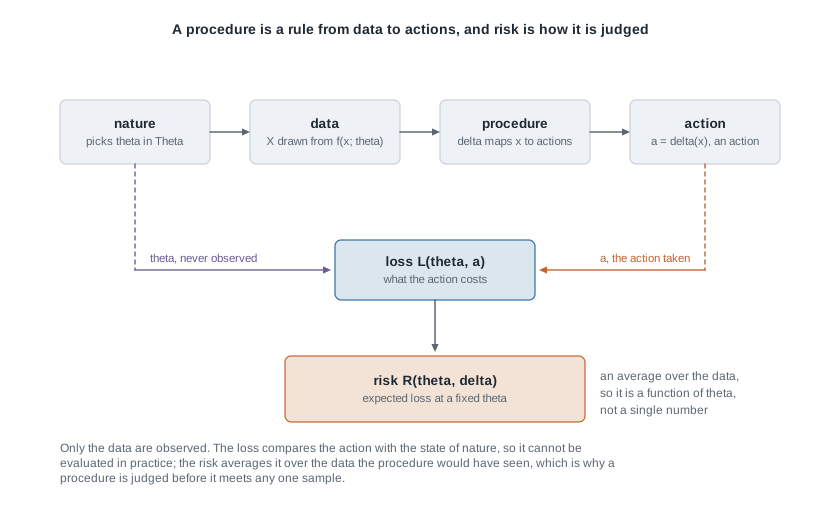
Read the diagram backwards from the risk box and the logic of the course appears. Risk averages over data the procedure has not seen, so it is a property of the rule and the model, never of the sample in front of you. That is why a procedure can be evaluated before any data exist, and why “this interval covers with probability 0.95” describes the recipe rather than the interval you hold.
From estimand to action space
The estimand and the action space are separate choices, and confusing them causes real errors. In point estimation of a normal mean an action is a number offered as the value of \(\theta\), so \(\mathcal{A} = \mathbb{R}\). In interval estimation an action is a subset of the parameter space, so \(\mathcal{A}\) is a collection of intervals and the loss must price both width and failure to cover. In testing, which starts next week, \(\mathcal{A}\) has two elements and the loss prices the two errors. Nothing else about the model changes across the three settings.
The procedure must be a function of the data alone. That sounds obvious and is violated constantly in disguise: an expression involving \(\theta\) is not a procedure, however well it performs. The trap appears explicitly in the first worked example, where the best shrinkage constant depends on the parameter being estimated, so the object with the lowest risk curve is unusable.
Loss functions and the actions they select
Three losses cover most of what this course needs. Squared-error loss \(L(\theta, a) = (\theta - a)^2\) penalizes large errors quadratically and splits neatly into a variance and a squared bias. Absolute-error loss \(L(\theta, a) = |\theta - a|\) penalizes proportionally and is far less sensitive to one rare large error. Zero-one loss \(L(\theta, a) = \mathbf{1}\{a \ne \theta\}\) prices only whether the action is exactly right, which suits a parameter space of finitely many labels.
Suppose the information about \(\theta\) has been reduced to a distribution over \(\Theta\) — in a Bayesian problem the posterior given the data — and write \(E[\cdot]\) for expectation under it. The action minimizing expected loss is then fixed by the loss alone, under conditions worth stating.
- Squared error. \(E[(\theta - a)^2] = \operatorname{Var}(\theta) + (E[\theta] - a)^2\), minimized uniquely at \(a = E[\theta]\). This needs \(E[\theta^2] < \infty\); with no second moment every action has infinite expected loss and the criterion says nothing.
- Absolute error. Provided \(E|\theta| < \infty\), the map \(a \mapsto E|\theta - a|\) is convex with right derivative \(P(\theta \le a) - P(\theta > a)\) and left derivative \(P(\theta < a) - P(\theta \ge a)\), so the minimizers are exactly the points where the first is non-negative and the second non-positive: the medians. The minimizer is unique when the distribution function is strictly increasing there, and an interval otherwise.
- Zero-one. For continuous \(\theta\) the strict form is useless: every action has expected loss one. Replace it by \(L_\epsilon(\theta, a) = \mathbf{1}\{|\theta - a| > \epsilon\}\), with expected loss \(1 - P(|\theta - a| \le \epsilon)\), so the best action centres a window of width \(2\epsilon\) on the most probable region. If the density is continuous with a unique maximum, shrinking \(\epsilon\) to zero drives that action to the mode. On a finite parameter space the mode is optimal outright, with no limit needed.
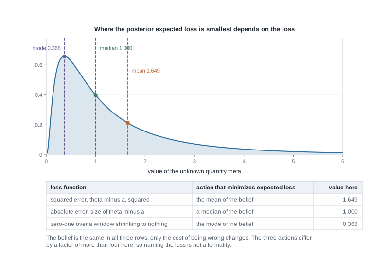
The figure makes the size of the effect concrete. Take the belief in which \(\log\theta\) is standard normal, so \(\theta\) is positive and right-skewed: its mode is \(e^{-1} = 0.368\), its median is \(1\), its mean is \(e^{1/2} = 1.649\). Three defensible losses, one unchanged belief, three actions differing by a factor of more than four. A report giving an estimate without naming the loss has still chosen one, silently.
Risk as a function of the parameter
Averaging the loss over the data at a fixed parameter value gives the risk. The squared-error case is used relentlessly, so write it out: for any estimator \(\delta\) of \(\theta\),
\[ R(\theta, \delta) \;=\; E_\theta (\theta - \delta(X))^2 \;=\; \operatorname{Var}_\theta \delta(X) \;+\; \bigl( E_\theta \delta(X) - \theta \bigr)^2 , \]
the familiar decomposition into variance and squared bias, now read as an identity between functions of \(\theta\) rather than between numbers. Both terms move with \(\theta\), and typically in opposite directions, which is exactly why risk curves cross.
Domination, admissibility, and a partial order
Risk induces an ordering on procedures, and it is worth being precise about how weak that ordering is. Say \(\delta_1\) dominates \(\delta_2\) when \(R(\theta, \delta_1) \le R(\theta, \delta_2)\) for every \(\theta \in \Theta\), with strict inequality for at least one \(\theta\); a procedure is admissible when nothing dominates it. Notice what the definition demands: an inequality at every point of the parameter space. Two curves that cross satisfy it in neither direction, so the pair is not ranked at all. This is a partial order, and the incomparable case is the common one.
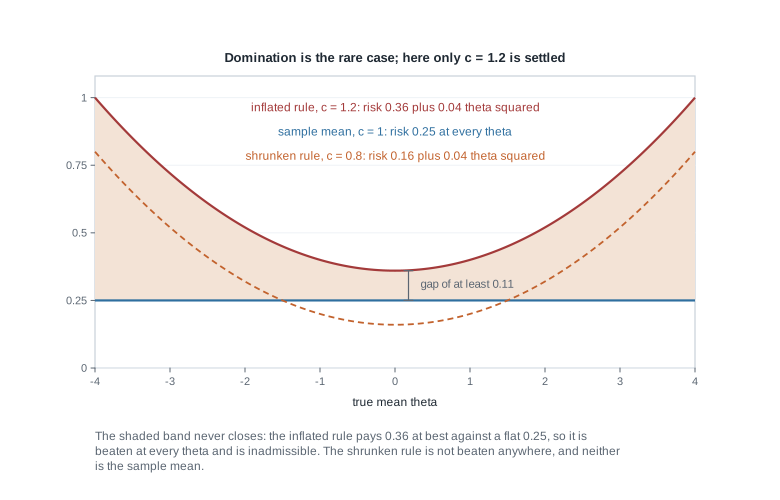
The figure shows both cases at once, for the rules \(\delta_c(X) = c\bar{X}\) developed below. The curve for \(c = 1.2\) never falls below \(0.36\) while the sample mean’s risk is \(0.25\) everywhere, so the gap never closes and \(c = 1.2\) is inadmissible. The curve for \(c = 0.8\) crosses the flat line, so that pair stays unsettled.
The two properties are worth very different amounts. Inadmissibility is a genuine defect: a dominated procedure can be replaced by one at least as good everywhere and better somewhere, at no cost. Admissibility promises almost nothing. In the normal model with known variance and squared-error loss, the rule that ignores the data and always reports \(17\) is admissible: its risk \((\theta - 17)^2\) is zero at \(\theta = 17\), so any competitor with risk no larger everywhere must have zero risk there, forcing it to equal \(17\) with probability one under \(P_{17}\) and hence under every \(P_\theta\), since normal densities with a common variance share the same null sets. Nothing dominates it, and it is still useless. Admissibility screens; it does not recommend.
Collapsing a risk function to a number
Because the partial order settles so little, the common move is to collapse each risk curve into one number and rank those. Two standard ways exist, and they answer different questions. The Bayes risk against a prior \(\pi\) is the weighted average \(r(\pi, \delta) = \int_\Theta R(\theta, \delta) \, \pi(d\theta)\), asking how the procedure does across parameter values weighted by how plausible you find them. The maximum risk \(\sup_{\theta \in \Theta} R(\theta, \delta)\) asks how badly it can do at its worst parameter value, with no weighting at all.
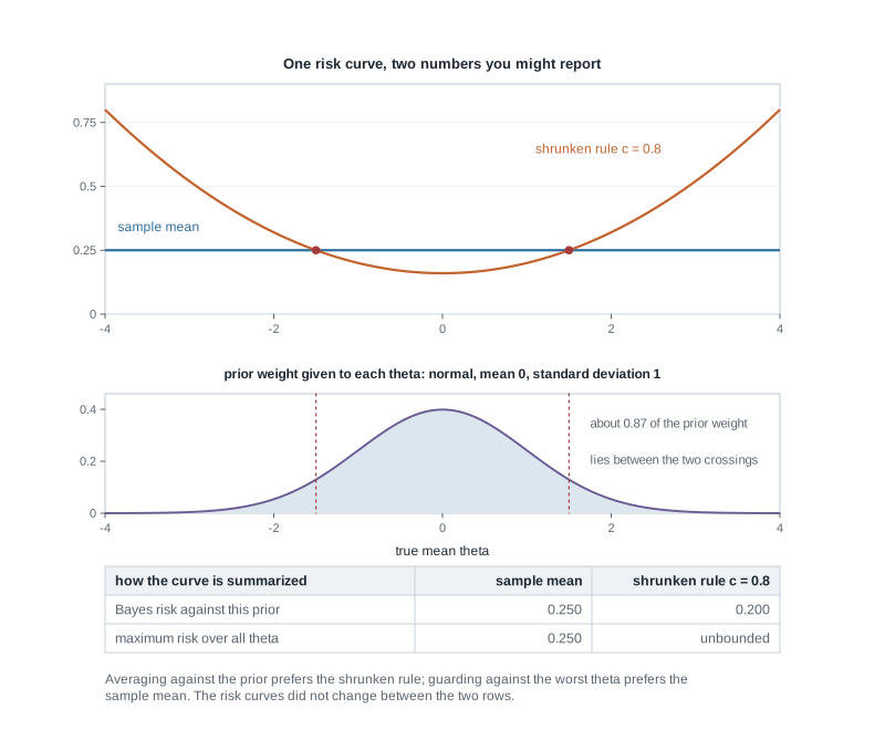
The figure previews how sharply they can disagree. Averaged against a standard normal prior the shrunken rule wins, \(0.200\) against \(0.250\); judged by its worst case it loses outright, since its risk grows without bound as \(|\theta|\) grows while the sample mean’s stays flat. Neither curve changed between those verdicts — only the question did. Both summaries return as machinery in Week 14; for now treat them as two honest and non-equivalent ways of reducing a function to a number.
Worked example — a normal mean under squared-error loss
The model and the question. Let \(X_1, \dots, X_{16}\) be independent \(N(\theta, \sigma^2)\) with \(\sigma^2 = 4\) known and \(\theta\) unknown in \(\Theta = \mathbb{R}\). The estimand is \(\theta\), the action space is the real line, and the loss is squared error. Compare the sample mean \(\delta_1(X) = \bar{X}\) with the shrunken rule \(\delta_c(X) = c\bar{X}\) for a constant \(c\) fixed in advance.
Step 1: the sampling distribution. With \(n = 16\) and \(\sigma^2 = 4\) we have \(\bar{X} \sim N(\theta, \sigma^2/n)\), so \(\operatorname{Var}_\theta \bar{X} = 4/16 = 0.25\) and the standard error is \(0.5\). Write \(v = 0.25\) throughout.
Step 2: the risk of the sample mean. \(\bar{X}\) is unbiased, so the squared-bias term vanishes and \(R(\theta, \delta_1) = v = 0.25\) at every \(\theta\). That flat curve is what makes this pair easy to draw.
Step 3: the risk of the shrunken rule. Here \(E_\theta \delta_c = c\theta\), so the bias is \((c - 1)\theta\), and \(\operatorname{Var}_\theta \delta_c = c^2 v\). The decomposition gives
\[ R(\theta, \delta_c) \;=\; c^2 v \;+\; (1 - c)^2 \theta^2 \;=\; 0.16 \;+\; 0.04\,\theta^2 \quad \text{at } c = 0.8 . \]
Step 4: where each rule wins. Setting the risks equal, \(c^2 v + (1-c)^2\theta^2 = v\) gives \((1-c)^2\theta^2 = (1 - c^2)v\), and cancelling one factor of \(1 - c\) — legitimate because \(c < 1\) — leaves \(\theta^2 = v(1 + c)/(1 - c)\). At \(c = 0.8\) that is \(0.25 \times 9 = 2.25\), so the curves cross at \(\theta = \pm 1.5\), three standard errors from zero. Inside that range shrinking helps: at \(\theta = 0\) the risk falls from \(0.25\) to \(0.16\), down thirty-six percent. Outside it shrinking hurts: at \(\theta = 3\) the risk is \(0.16 + 0.04 \times 9 = 0.52\), more than twice the sample mean’s.
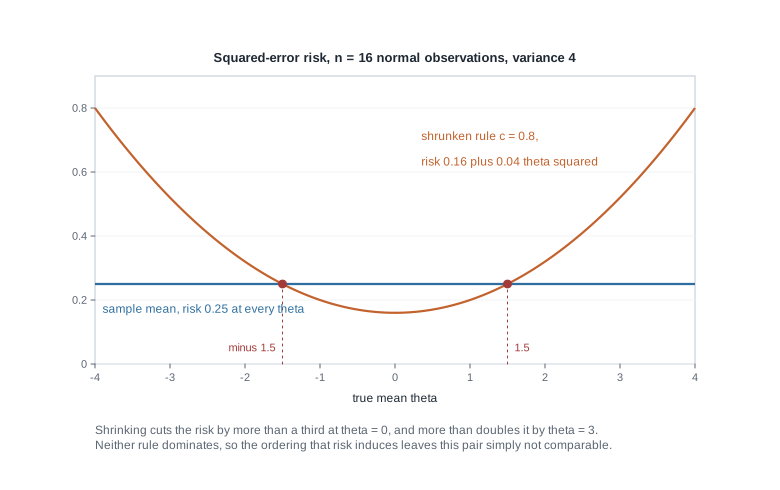
Step 5: could a better constant be chosen? Minimizing \(c^2 v + (1-c)^2\theta^2\) over \(c\) gives \(c^\ast(\theta) = \theta^2/(\theta^2 + v)\) with risk \(v\theta^2/(\theta^2 + v)\), strictly below \(v\) at every \(\theta\). That looks like a rule dominating the sample mean and is not one, because \(c^\ast\) depends on the unknown \(\theta\) while a procedure must be a function of the data alone. At \(\theta = 1\) the best constant is \(0.8\); at \(\theta = 3\) it is \(0.973\). Choosing a constant after seeing where the truth lies is hindsight, not a procedure.
v <- 4 / 16                                   # variance of the sample mean, sigma^2 / n
risk_shrunk <- function(theta, c) c^2 * v + (1 - c)^2 * theta^2
theta <- seq(-4, 4, by = 0.01)

plot(theta, rep(v, length(theta)), type = "l", ylim = c(0, 0.9),
     xlab = "theta", ylab = "risk under squared-error loss")
lines(theta, risk_shrunk(theta, 0.8), lty = 2)
lines(theta, risk_shrunk(theta, 1.2), lty = 3)
sqrt(v * (1 + 0.8) / (1 - 0.8))               # 1.5, the crossing
What this licenses and what it does not. Neither \(\delta_1\) nor \(\delta_{0.8}\) dominates, so the risk ordering does not choose between them and no further computation will. Both are in fact admissible. For \(\delta_{0.8}\) the argument is short: under the prior \(\theta \sim N(0, \tau^2)\) the posterior mean is \(\tau^2\bar{x}/(\tau^2 + v)\), which equals \(0.8\bar{x}\) when \(\tau^2 = 1\), so \(\delta_{0.8}\) is the Bayes rule for the standard normal prior under squared-error loss. A Bayes rule with finite Bayes risk that is essentially unique is admissible, since a dominating rule would have Bayes risk no larger and would therefore be Bayes too, contradicting uniqueness. Its Bayes risk is \(0.16 + 0.04 \, E_\pi[\theta^2] = 0.20\), matching the posterior variance \(\tau^2 v/(\tau^2 + v) = 0.2\) as it must. That \(\bar{X}\) is itself admissible here is true but harder, needing a limiting argument over priors, and the corresponding statement fails in three or more dimensions — the Stein phenomenon, stated carefully in Week 14.
The same reasoning, transferred
Now let \(X_1, \dots, X_{20}\) be independent Poisson with mean \(\theta > 0\), counting surface defects per inspected panel, and compare \(\bar{X}\) with \(\delta_c = c\bar{X}\) under squared-error loss again. Here \(\operatorname{Var}_\theta \bar{X} = \theta/20\), so \(R(\theta, \bar{X}) = 0.05\,\theta\) and \(R(\theta, \delta_c) = c^2\theta/20 + (1-c)^2\theta^2\), which at \(c = 0.8\) is \(0.032\,\theta + 0.04\,\theta^2\). Equating and cancelling one factor of \(\theta\) gives \(0.04\,\theta = 0.018\), so the curves cross once, at \(\theta = 0.45\).
What stayed the same is the whole skeleton: \(c^2\) times a variance plus \((1-c)^2\) times a squared bias, shrinkage winning where the parameter is small relative to the noise, and the same one-line argument that any \(c > 1\) is dominated by \(c = 1\), since \((c^2 - 1)\theta/20 + (1-c)^2\theta^2 > 0\) for every \(\theta > 0\). What changed is that the variance now depends on \(\theta\), so the sample mean’s risk is no longer flat; the parameter space is a half-line, so there is one crossing rather than a symmetric pair.
Second worked example — accepting or rejecting a batch under asymmetric loss
The model and the question. A supplier delivers a batch of six hundred units of which an unknown proportion \(\theta\) are defective. The action space has two elements: accept, or reject and re-source. Each defective unit that ships costs three dollars in warranty and replacement, so accepting costs \(1800\,\theta\) dollars on average, while rejecting costs a flat one hundred and fifty dollars whatever \(\theta\) turns out to be. The loss is
\[ L(\theta, \text{accept}) = 1800\,\theta , \qquad L(\theta, \text{reject}) = 150 , \]
asymmetric in the strong sense that the two costs are different functions of \(\theta\), not merely different constants.
Step 1: what full information would do. If \(\theta\) were known, accepting is cheaper exactly when \(1800\theta < 150\), that is when \(\theta < 1/12 \approx 0.0833\). Call \(\theta^{\dagger} = 1/12\) the break-even defect rate. An oracle’s loss is \(\min(1800\theta, 150)\), and no procedure’s risk can fall below that curve.
Step 2: the data. Inspect \(n = 25\) units and let \(X\) be the number defective. Drawing twenty-five units from six hundred without replacement is strictly hypergeometric, but the inspected fraction is small enough that \(X \sim \text{Binomial}(25, \theta)\) is the usual approximation; note the swap now so it can be checked later.
Step 3: the optimal action. Put a \(\text{Beta}(2, 18)\) prior on \(\theta\), centred at \(0.1\) and worth about twenty observations. Given \(X = x\) the posterior is \(\text{Beta}(2 + x, \, 43 - x)\), with mean \((2 + x)/45\). The expected loss of accepting is \(1800 \, E[\theta \mid x]\) and of rejecting is \(150\), so rejecting is optimal when
\[ E[\theta \mid x] \;=\; \frac{2 + x}{45} \;>\; \frac{150}{1800} \;=\; \frac{1}{12} . \]
Because the loss is linear in \(\theta\), the posterior enters only through its mean; under a loss nonlinear in \(\theta\) that reduction fails and the whole posterior is needed.
Step 4: the rule this produces. The inequality \((2 + x)/45 > 1/12\) is \(2 + x > 3.75\), that is \(x \ge 2\). The optimal procedure is the familiar acceptance-sampling rule: reject if at least two of the twenty-five inspected units are defective. With \(x = 3\) the posterior mean is \(5/45 = 0.111\), above the break-even rate, so the batch is rejected.
Step 5: how the cutoff moves with the loss ratio. Replace the rejection cost by a general \(C\). Rejecting is optimal when \((2 + x)/45 > C/1800\), that is \(x > C/40 - 2\), so the cutoff depends on the loss ratio and the prior and on nothing else.
| cost \(C\) of rejecting | break-even rate \(C/1800\) | reject when | action at \(x = 3\) |
|---|---|---|---|
| 150 | 0.0833 | \(x \ge 2\) | reject |
| 200 | 0.1111 | \(x \ge 4\) | indifferent |
| 250 | 0.1389 | \(x \ge 5\) | accept |
Step 6: the risk function of the rule. Write \(\delta_k\) for “reject if \(X \ge k\)”. At \(C = 150\),
\[ R(\theta, \delta_k) \;=\; 1800\,\theta \; P_\theta(X \le k - 1) \;+\; 150 \; P_\theta(X \ge k) . \]
Every such curve passes through \((1/12, \, 150)\): at the break-even rate the two actions cost the same, so what the rule does there cannot matter. Away from it the curves separate. At \(\theta = 0.05\) the risk of \(\delta_2\) is \(111.5\) dollars against \(90.4\) for \(\delta_5\), oracle floor \(90.0\); at \(\theta = 0.15\) the ranking reverses, \(161.2\) against \(231.9\), floor \(150\). Two procedures, no winner.
n <- 25; K <- 1800; C <- 150
post_mean <- function(x) (2 + x) / 45          # Beta(2, 18) prior, 25 inspected units
min(which(post_mean(0:n) > C / K)) - 1         # 2, the first count that rejects

risk_k <- function(theta, k) {
  p_accept <- pbinom(k - 1, n, theta)
  K * theta * p_accept + C * (1 - p_accept)
}
risk_k(c(0.05, 1/12, 0.15), 2)                 # 111.46  150.00  161.17
risk_k(c(0.05, 1/12, 0.15), 5)                 #  90.43  150.00  231.85
What this licenses and what it does not. Collapsing the curves confirms the construction: against the \(\text{Beta}(2, 18)\) prior the Bayes risk of \(\delta_2\) is \(130.9\) dollars against \(149.2\) for \(\delta_5\), as it must be, since \(\delta_2\) minimizes posterior expected loss at every \(x\) and therefore minimizes the average of the risk curve. Their maximum risks are \(162.2\) and \(241.0\) dollars, so here the two summaries agree; the normal example shows they need not. What none of this licenses is treating the cutoff as a property of the data. It belongs to the loss ratio and the prior, and a report giving it without them has hidden its two most contestable inputs.
The misreading to avoid
The misreading, in the words graduate students actually use, is this: “the shrunken estimator has smaller mean squared error, so it is the better estimator.” Smaller than what, and where? The shrunken rule above has mean squared error \(0.16\) against \(0.25\) at \(\theta = 0\), and \(0.52\) against \(0.25\) at \(\theta = 3\). The sentence is true at one parameter value and false at another, and it feels complete only because the notation \(\text{MSE}(\hat\theta)\) suppresses the argument that makes it a function. Write \(R(\theta, \delta)\) and the error becomes hard to commit.
The dismantling has three parts. Risk is a function on \(\Theta\), so a comparison is a comparison of functions, and the only one the definition supports is domination, an inequality at every point. Most pairs are incomparable, which is a fact about the ordering rather than a failure of your analysis; when two curves cross, the honest report is that they cross, and where. And a single verdict requires supplying the extra ingredient that produces one — a prior, giving Bayes risk, or a worst-case stance, giving maximum risk — and naming which you used, since the two disagree in exactly the cases where it matters.
Two smaller misreadings travel with the large one. The first reads risk as what you will lose on the data set in front of you. It is an average over repeated data at a fixed parameter value, so a procedure with excellent risk can do badly on your sample and you will never learn which happened. The second treats admissibility as approval, when the constant rule reporting \(17\) is admissible and useless, while inadmissibility is genuinely informative because the improvement it promises costs nothing.
Practice on your own
These are for self-checking as you read, not for submission. Work them with a pencil first, then with R.
- The full family of shrinkage constants. For \(X_1, \dots, X_n\) independent \(N(\theta, \sigma^2)\) with \(\sigma^2\) known, derive \(R(\theta, \delta_c)\) for arbitrary real \(c\), then show every \(c > 1\) is dominated by \(c = 1\) and every \(c < 0\) by \(c = 0\). For \(c\) in \([0, 1]\), identify the prior making \(\delta_c\) a Bayes rule, and state the condition on the Bayes risk the admissibility argument needs.
- The same estimators under a different loss. Redo the comparison of \(\bar{X}\) and \(0.8\bar{X}\) under absolute-error loss with \(\bar{X} \sim N(\theta, 0.25)\). Show \(E_\theta|\bar{X} - \theta| = 0.5\sqrt{2/\pi} \approx 0.399\), constant in \(\theta\), evaluate the shrunken rule at \(\theta = 0\) and \(\theta = 3\), and say whether the crossing moves inward or outward.
- A loss for which the mean is wrong. With \(\log\theta\) standard normal, take the loss equal to \(2(\theta - a)\) when \(a \le \theta\) and \(a - \theta\) when \(a > \theta\). Show the optimal action is a quantile of the belief, identify which one, and compare it with the mean \(1.649\) and the median \(1\).
- Moving the cutoff. Redo the batch problem with a \(\text{Beta}(1, 1)\) prior, obtain the cutoff for \(C = 150\) and for \(C = 250\), and confirm numerically that every risk curve still passes through \((1/12, 150)\). Say in one sentence why that holds for any procedure whatsoever.
- A simulated risk curve. Estimate \(R(\theta, \bar{X})\) and \(R(\theta, 0.8\bar{X})\) by simulation on a grid from \(-4\) to \(4\) with twenty thousand replicates each, plot both, and locate the crossing. Report the Monte Carlo standard error at \(\theta = 1.5\) and say whether it resolves the crossing.
Where to read more
- MIT OpenCourseWare 18.655 Mathematical Statistics opens with this framing of models, decision rules, loss, and risk, and its early lecture notes are the closest open match to this week.
- Penn State STAT 415 Introduction to Mathematical Statistics is the gentler open reference; use it to refresh the variance-plus-squared-bias decomposition or elementary Bayes estimators if either felt shaky above.
- The optional Hogg, McKean, and Craig alignment for this week is Chapter 8.5, together with Chapter 11.1 through 11.2. The text is optional throughout this course and is never required to be purchased; availability and licence terms for every source listed here are still being confirmed.
- Computing needs nothing beyond The R Project for Statistical Computing and Quarto; base R draws every curve on this page.
- The course pages: the syllabus, the schedule, the resources overview, and the notes index. The prerequisite review is Week 0 — Readiness review from Mathematical Statistics I.
Where this goes next
Week 2 specializes all of this to an action space with two elements. A hypothesis test is a decision problem in which \(\Theta\) splits into \(\Theta_0\) and \(\Theta_1\), the actions are reject and do not reject, and the loss prices the two errors separately. The risk function becomes the pair of error probabilities, the power function \(\beta(\theta) = E_\theta \varphi\) takes the place of the risk curve, and the Neyman-Pearson lemma settles, for a simple null against a simple alternative, the question this week could not: which procedure is best. It settles it by fixing one error probability and optimizing the other, which breaks the tie rather than showing it was illusory.
Read Week 2 — Tests as decision rules and the Neyman-Pearson lemma next, and return to the notes index for the full sequence. Keep this week’s picture in view all term: when a later unit compares an exact procedure with an approximation, a robust estimator with the mean, or a Bayes rule with a frequentist one, it is comparing risk functions, and the comparison usually ends in a crossing rather than a winner.