Week 8 — Normal linear models, projections, and quadratic forms
Where this week starts
Weeks 5 and 6 handed you three statistics that share a limiting distribution, and Week 7 asked whether that limit had arrived at the sample size in front of you. Most of the first half’s guarantees are approximate. This week is the exception the course has been saving: for the normal linear model with independent errors of common variance, the distribution of everything the procedure reports is known exactly, at every sample size, with no appeal to a limit. Twelve observations are enough, and so are five.
The reason is geometric, and it fits in a sentence: least squares is an orthogonal projection, and the normal law with covariance \(\sigma^2 I\) is the one law that does not notice a rotation. The rest follows. Fitted values are a projection onto a subspace; sums of squares are squared lengths; degrees of freedom are ranks; independence of two sums of squares is orthogonality of two subspaces. The \(t\) and \(F\) statistics are ratios of those pieces from which the unknown \(\sigma^2\) cancels, which is what makes them pivotal.
What should feel different by the end is how you read an analysis-of-variance table: not as a bookkeeping convention, but as one vector in \(\mathbb{R}^n\) resolved into orthogonal components, with the rank of each in the degrees-of-freedom column and its squared length beside it. Model building and diagnostics belong to the regression course; this week stays on the theory that licenses them, and closes by asking what happens when the covariance assumption fails.
Why this matters beyond the theorem
Here is the stake. A field trial with three treatments and four plots each gives a ratio of mean squares of 9.00 on 2 and 9 degrees of freedom, tail probability 0.0071, and a report goes out claiming a treatment effect. Now suppose the four plots within a treatment shared an irrigation channel, so observations within a group are correlated with \(\rho = 0.3\). Every number is computed identically, both sums of squares are still independent chi-squares, and the ratio is still called \(F\). Its actual null distribution, derived below, is 2.71 times an \(F_{2,9}\), so the test advertising level 0.05 has actual size 0.26. The output never complains, and more plots per treatment make it worse.
The second stake is quieter. Write the one-way model as \(\mu + \alpha_i\) and you have written four parameters for a three-dimensional subspace. Count parameters and the between-groups degrees of freedom come out as 3; take the rank of the projection and they come out as 2. Every \(F\) ratio downstream depends on which you used, and only one is a property of the model rather than of the notation.
What you will be able to do
- Derive the hat matrix for a stated design and verify that it is symmetric, idempotent, and of rank equal to its trace.
- State and prove the distribution of a quadratic form in a normal vector, naming which conclusion fails when idempotence, the covariance \(\sigma^2 I\), or the centring is dropped.
- Decompose a one-way layout into orthogonal projections, give each component’s degrees of freedom as a rank, and check Cochran’s rank condition arithmetically.
- Construct \(t\) and \(F\) from the geometry instead of quoting them, and show \(t^2 = F\) whenever the numerator has one degree of freedom.
- Diagnose which assumption a linear-model conclusion rests on, and compute the true size of an \(F\) test when the error covariance is not \(\sigma^2 I\).
- Verify a claimed quadratic-form distribution by simulation.
Terms and notation worth fixing
| Symbol | What it means on this page |
|---|---|
| \(X\) | The \(n \times p\) design matrix, fixed and known, of full column rank \(p\) unless stated otherwise |
| \(V = \mathcal{C}(X)\) | The model subspace: the column space of \(X\), the mean vectors the model permits |
| \(P\) | The hat matrix \(X(X^{\top}X)^{-1}X^{\top}\), orthogonal projection onto \(V\), so \(\hat{y} = Py\) |
| \(V_0\), \(P_0\) | The null subspace and its projection; here \(V_0\) is always a subspace of \(V\) |
| \(\operatorname{rank}(A)\) | Dimension of the range of \(A\); for a projection it equals \(\operatorname{tr}(A)\), and it is what “degrees of freedom” names |
| \(\chi^2_r(\lambda)\) | Chi-square on \(r\) degrees of freedom with noncentrality \(\lambda\), mean \(r + \lambda\); the central case is \(\chi^2_r\), and note that this \(\lambda\) is twice the noncentrality parameter Hogg, McKean, and Craig write for the same law |
| \(F_{q,m}\) | The law of \((\chi^2_q / q)/(\chi^2_m / m)\) with the two parts independent |
| \(\sigma^2\) | The common error variance, estimated by \(\hat\sigma^2 = \lVert (I - P)y \rVert^2/(n - p)\) |
Least squares as an orthogonal projection
Fix the model for the week. Let \(Y = X\beta + \varepsilon\) with \(Y\) an \(n\)-vector, \(X\) a known \(n \times p\) matrix, \(\beta \in \mathbb{R}^p\) unknown, and \(\varepsilon \sim N_n(0, \sigma^2 I_n)\). Three assumptions are bundled there, and different conclusions need different subsets of them: the mean vector lies in \(V = \mathcal{C}(X)\); the errors are uncorrelated with common variance; the errors are normal. Least squares itself needs none of the three, since minimizing \(\lVert y - Xb \rVert^2\) is linear algebra. Unbiasedness needs the first, the usual variance formula the first two, and the exact chi-square, \(t\), and \(F\) laws all three.
The minimization has a one-line geometric reading. Among vectors in \(V\) we want the one closest to \(y\), and the closest point of a subspace is the orthogonal projection onto it. Equivalently the residual must be orthogonal to every column of \(X\), which is the normal equations \(X^{\top}(y - X\hat\beta) = 0\). With full column rank, \(X^{\top}X\) is invertible, \(\hat\beta = (X^{\top}X)^{-1}X^{\top}y\), and \(\hat{y} = Py\) with \(P = X(X^{\top}X)^{-1}X^{\top}\).
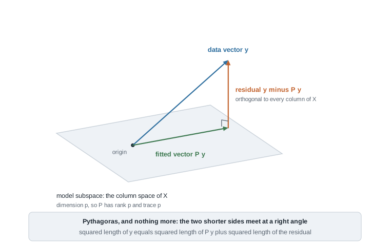
Keep that picture in view: the plane is \(V\), the right angle at the foot of the residual is the normal equations, and the Pythagorean identity in the panel is the sum-of-squares decomposition, written down before any probability has entered the argument.
The hat matrix and what idempotence buys
Two properties of \(P\) do the work. It is symmetric, because \((X^{\top}X)^{-1}\) is symmetric and transposing the product returns it unchanged. It is idempotent:
\[ P^2 = X(X^{\top}X)^{-1}X^{\top}X(X^{\top}X)^{-1}X^{\top} = X(X^{\top}X)^{-1}X^{\top} = P , \]
which is the algebraic form of an obvious geometric fact — a vector already in \(V\) is its own projection. The eigenvalues follow at once. If \(Pv = \lambda v\) with \(v \ne 0\), then \(\lambda v = P^2 v = \lambda^2 v\), so \(\lambda\) is 0 or 1. A symmetric matrix is diagonalizable by an orthogonal matrix, so the number of unit eigenvalues is the rank, and since the trace is the sum of the eigenvalues, \(\operatorname{rank}(P) = \operatorname{tr}(P)\). Here that number is \(p\), because \(\operatorname{tr}\{X(X^{\top}X)^{-1}X^{\top}\} = \operatorname{tr}\{(X^{\top}X)^{-1}X^{\top}X\} = p\) by cyclic invariance of the trace.
One consequence is the reason degrees of freedom are ranks. Replace \(X\) by \(\tilde{X} = XA\) for an invertible \(p \times p\) matrix \(A\) — what happens when you recode a factor or centre a covariate. Then
\[ \tilde{P} = XA(A^{\top}X^{\top}XA)^{-1}A^{\top}X^{\top} = XAA^{-1}(X^{\top}X)^{-1}(A^{\top})^{-1}A^{\top}X^{\top} = P . \]
The projection, the fitted values, the residuals, the sums of squares, and their ranks are properties of \(V\) alone. The coefficient vector \(\hat\beta\) is not; it is a set of coordinates. When \(X\) is rank deficient — the one-way model with an intercept and one indicator per group — \(\hat\beta\) is not even unique, while \(P\) and every sum of squares still are, and \(\operatorname{rank}(P) = \operatorname{rank}(X)\) is smaller than the number of columns. That rank belongs in the table.
Finally \(I - P\) is symmetric and idempotent of rank \(n - p\), projecting onto \(V^{\perp}\). The residual is \(e = (I - P)y\), and since \(PX = X\) we get \(E e = 0\) for every \(\beta\). The diagonal entries \(h_{ii} = P_{ii}\) are the leverages, and they sum to \(\operatorname{tr}(P) = p\).
Sums of squares are squared lengths
Because \(y = Py + (I - P)y\) with orthogonal pieces, Pythagoras gives \(\lVert y \rVert^2 = \lVert Py \rVert^2 + \lVert (I - P)y \rVert^2\), and every finer decomposition is the same trick inside a nested pair of subspaces.
Suppose the hypothesis says the mean lies in a smaller subspace \(V_0 \subseteq V\) of dimension \(p_0 < p\). Because \(V_0\) sits inside \(V\), projecting onto \(V_0\) and then onto \(V\) changes nothing: \(P P_0 = P_0\), and transposing gives \(P_0 P = P_0\). Hence
\[ (P - P_0)^2 = P^2 - PP_0 - P_0P + P_0^2 = P - P_0 - P_0 + P_0 = P - P_0 , \]
so \(P - P_0\) is symmetric and idempotent of rank \(p - p_0\): it projects onto the part of \(V\) orthogonal to \(V_0\). The identity the week runs on is therefore
\[ I_n = P_0 + (P - P_0) + (I - P) , \qquad p_0 + (p - p_0) + (n - p) = n . \]
Apply each piece to \(y\) and take squared lengths: three orthogonal components whose squared lengths add, with ranks adding to \(n\). When \(V_0\) is the span of the vector of ones, dropping the first term is what correcting for the mean does, and the two that remain are the between and within lines of an analysis-of-variance table.
Quadratic forms in a normal vector
Every sum of squares above is \(Y^{\top}AY\) for a symmetric idempotent \(A\), since \(\lVert AY \rVert^2 = Y^{\top}A^{\top}AY = Y^{\top}AY\). The distribution theory therefore reduces to two questions: what is the law of such a form, and when are two of them independent?
The chi-square theorem and its conditions
Theorem. Let \(Z \sim N_n(0, I_n)\) and let \(A\) be symmetric and idempotent with \(\operatorname{rank}(A) = r\). Then \(Z^{\top}AZ \sim \chi^2_r\).
Working. Symmetry gives \(A = Q \Lambda Q^{\top}\) with \(Q\) orthogonal and \(\Lambda\) diagonal. Idempotence forces each diagonal entry to satisfy \(\lambda^2 = \lambda\), so exactly \(r\) of them equal one. Put \(W = Q^{\top}Z\); then \(W\) is normal with mean zero and covariance \(Q^{\top}Q = I\), which is where \(\operatorname{Cov}(Z) = I\) earns its place, since the standard normal is the law unchanged by an orthogonal change of basis. Finally \(Z^{\top}AZ = W^{\top}\Lambda W = \sum_{i=1}^{r} W_i^2\), a sum of \(r\) independent squared standard normals, which is \(\chi^2_r\) by definition.
Both conditions are load-bearing. Drop idempotence and the eigenvalues are arbitrary, so the form is \(\sum_i \lambda_i W_i^2\), a weighted sum of one-degree-of-freedom chi-squares, which is not a chi-square unless the nonzero weights are equal. Take \(A = \operatorname{diag}(1, 4)\) with \(n = 2\): the form \(Z_1^2 + 4Z_2^2\) has mean 5 and variance \(2(1)^2 + 2(4)^2 = 34\), whereas any \(\chi^2_r\) with mean 5 has variance 10. Symmetry costs nothing to assume, since \(Z^{\top}AZ = Z^{\top}\{(A + A^{\top})/2\}Z\).
Two extensions reach the models we use. If \(Y \sim N_n(\mu, \sigma^2 I_n)\) then \(Z = (Y - \mu)/\sigma\) is standard, so \((Y - \mu)^{\top}A(Y - \mu)/\sigma^2 \sim \chi^2_r\): the theorem is about the centred form. Uncentred, the law is noncentral, \(Y^{\top}AY/\sigma^2 \sim \chi^2_r(\lambda)\) with \(\lambda = \mu^{\top}A\mu/\sigma^2\), central exactly when \(A\mu = 0\). Check that condition every time. The within-groups sum of squares is central whatever the treatment means are, because \((I - P)X\beta = 0\) for every \(\beta\); the between-groups sum of squares is central only under the null, and its noncentrality \(\lambda = \lVert (P - P_0)\mu \rVert^2/\sigma^2\) is where the power function comes from.
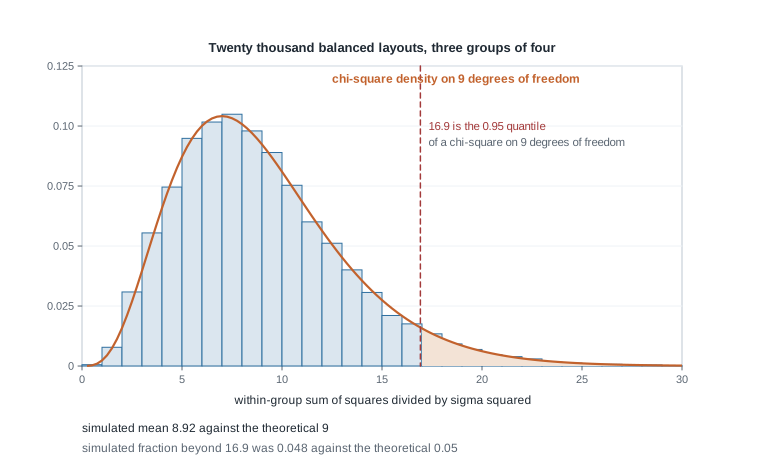
The figure checks the theorem: 20,000 simulated balanced layouts of three groups of four standard normal observations, with the within-groups sum of squares computed on each. The theorem predicts \(\chi^2_9\), mean 9 and variance 18. That run gave mean 8.92, variance 17.7, and 4.78 percent of replicates beyond 16.9, the 0.95 quantile of \(\chi^2_9\), against a predicted 5 percent; your own run will differ in the second decimal place.
Independence and Cochran’s decomposition
Proposition. Let \(Y \sim N_n(\mu, \sigma^2 I_n)\) and let \(A\) and \(B\) be symmetric idempotent with \(AB = 0\). Then \(AY\) and \(BY\) are independent, and so are \(Y^{\top}AY\) and \(Y^{\top}BY\).
Working. The stacked vector \((AY, BY)\) is a linear map of \(Y\), hence jointly normal, and \(\operatorname{Cov}(AY, BY) = A(\sigma^2 I)B^{\top} = \sigma^2 AB = 0\). For jointly normal vectors, zero covariance is independence — a property of the normal family, not a general fact, and exactly the step non-normal errors destroy. Since \(Y^{\top}AY = \lVert AY \rVert^2\) is a function of \(AY\), the forms are independent too.
The condition \(AB = 0\) says the ranges of \(A\) and \(B\) are orthogonal subspaces, and our nested decomposition satisfies it: \((I - P)(P - P_0) = P - P_0 - P^2 + PP_0 = 0\). The within and between sums of squares are independent because the subspaces are orthogonal, not because the formulas look separate.
The general statement is Cochran’s theorem. Let \(Z \sim N_n(0, I_n)\) and suppose \(I_n = A_1 + \dots + A_k\) with each \(A_j\) symmetric of rank \(r_j\). If \(r_1 + \dots + r_k = n\), then every \(A_j\) is idempotent, the forms \(Z^{\top}A_jZ\) are mutually independent, and \(Z^{\top}A_jZ \sim \chi^2_{r_j}\). The rank condition is the whole hypothesis: symmetric matrices summing to the identity may overlap, and only when the ranks add to \(n\) is no room left for it. So the first thing to do with a decomposition is add the ranks.
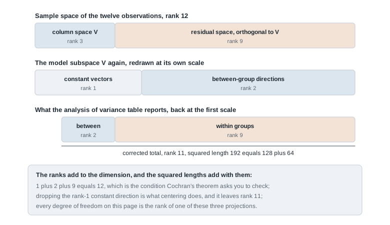
Read the figure as three views of one identity: the sample space split into the model subspace and its complement; the model subspace reopened into the constant direction and the two the treatments add; and what the table prints, with the constant direction removed by centring and rank 2 and rank 9 adding to the corrected total’s rank 11.
Building t and F rather than quoting them
Assemble. Under the null that \(E Y \in V_0\), the numerator \(\lVert (P - P_0)Y \rVert^2/\sigma^2\) is \(\chi^2_q\) with \(q = p - p_0\), because \(P - P_0\) annihilates any mean in \(V_0\). The denominator \(\lVert (I - P)Y \rVert^2/\sigma^2\) is \(\chi^2_{n-p}\) whether or not the null holds, and the two are independent. Therefore
\[ F = \frac{\lVert (P - P_0)Y \rVert^2 / q}{\lVert (I - P)Y \rVert^2 / (n - p)} \sim F_{q,\, n-p} . \]
Notice what became of \(\sigma^2\): it divides both sums of squares and cancels, so the null distribution carries no unknown parameter — Week 4’s definition of a pivot, reached by construction. Under an alternative with mean \(\mu \in V\) the numerator is noncentral with \(\lambda = \lVert (P - P_0)\mu \rVert^2/\sigma^2\), so power depends on the mean only through its distance from \(V_0\) in units of \(\sigma\).
The \(t\) statistic uses the same ingredients for a single linear combination. Fix \(c \ne 0\) and test \(c^{\top}\beta = \gamma_0\). Since \(c^{\top}\hat\beta\) is linear in \(Y\), it is normal with mean \(c^{\top}\beta\) and variance \(\sigma^2 c^{\top}(X^{\top}X)^{-1}c\); and \(\hat\beta\) is a function of \(PY\) while \(\hat\sigma^2\) is a function of \((I - P)Y\), so the proposition makes them independent. Standardizing both by the same \(\sigma\),
\[ t = \frac{c^{\top}\hat\beta - \gamma_0}{\hat\sigma \sqrt{c^{\top}(X^{\top}X)^{-1}c}} = \frac{N(0,1)}{\sqrt{\chi^2_{n-p}/(n-p)}} \sim t_{n-p} , \]
which is the definition of the \(t\) law. Squaring gives \(t^2 \sim F_{1, n-p}\). More is true than equality in distribution: for a one-dimensional hypothesis the numerator sum of squares equals \((c^{\top}\hat\beta - \gamma_0)^2 / \{c^{\top}(X^{\top}X)^{-1}c\}\), so \(t^2\) and \(F\) are the same number on every data set, as the second worked example checks.
Worked example — the one-way layout as two orthogonal projections
The model and the question. A field trial applies three fertilizer treatments to four plots each, with illustrative yields 9, 12, 14, 17 for treatment A; 15, 16, 18, 19 for treatment B; and 18, 20, 22, 24 for treatment C. Model them as \(Y_{ij} = \mu_i + \varepsilon_{ij}\) with \(\varepsilon_{ij}\) independent \(N(0, \sigma^2)\), \(i = 1, 2, 3\) and \(j = 1, \dots, 4\), so \(n = 12\). Test \(H_0 : \mu_1 = \mu_2 = \mu_3\) at level 0.05.
Step 1, name the two subspaces. \(V\) is spanned by the three group indicator vectors, which are linearly independent, so \(\dim V = 3\). \(V_0\) is spanned by the vector of ones, so \(\dim V_0 = 1\), and \(V_0 \subseteq V\) because a constant vector is a particular pattern of group means. That nesting licenses everything below.
Step 2, project. The group means are 13, 17, and 21, so \(Py\) repeats each group’s mean four times. The grand mean is \(204/12 = 17\), so \(P_0 y\) is 17 in every coordinate.
Step 3, take squared lengths. The between-groups component is
\[ \lVert (P - P_0)y \rVert^2 = \sum_{i=1}^{3} 4(\bar{y}_i - \bar{y})^2 = 4\{(-4)^2 + 0^2 + 4^2\} = 128 , \]
and the within-groups component is the sum of squared deviations inside each group: A gives \(16 + 1 + 1 + 16 = 34\), B gives \(4 + 1 + 1 + 4 = 10\), and C gives \(9 + 1 + 1 + 9 = 20\), totalling 64. The corrected total is \(\sum_{ij}(y_{ij} - 17)^2 = 98 + 10 + 84 = 192\), and \(128 + 64 = 192\) is Pythagoras in numbers.
Step 4, take ranks. \(\operatorname{rank}(P - P_0) = 3 - 1 = 2\) and \(\operatorname{rank}(I - P) = 12 - 3 = 9\); with the rank-1 constant direction the ranks are \(1 + 2 + 9 = 12\), which is Cochran’s condition.
Step 5, get the distributions. Under \(H_0\) the mean lies in \(V_0\) and is annihilated by \(P - P_0\), so \(128/\sigma^2\) is a draw from \(\chi^2_2\). The within component is central regardless, since \((I - P)\mu = 0\) for every \(\mu \in V\), so \(64/\sigma^2\) is a draw from \(\chi^2_9\). They are independent because \((I - P)(P - P_0) = 0\) and the errors are normal with covariance \(\sigma^2 I\).
Step 6, form the ratio. The mean squares are \(128/2 = 64\) and \(64/9 = 7.11\), so \(F = 64 \div (64/9) = 9.00\) on \(F_{2,9}\), and \(\hat\sigma = \sqrt{64/9} = 8/3 = 2.67\) on 9 degrees of freedom. For two numerator degrees of freedom the tail has the closed form \(P(F_{2,m} > f) = (1 + 2f/m)^{-m/2}\), so the tail probability is \((1 + 18/9)^{-4.5} = 3^{-4.5} = 0.0071\), and the same equation gives the 0.05 cutoff 4.26.
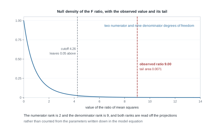
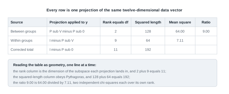
Step 7, what it licenses and what it does not. The table figure is the whole computation, each entry a projection. The result licenses a conditional statement: if the three means were equal and the model held, a discrepancy this large would arise about seven times in a thousand. It does not say which pair differs, since the numerator pools two dimensions into one number and discards the direction — that is Week 9’s question. And it is not evidence that the model is correct: a small tail probability is equally consistent with unequal means and with a violated covariance assumption.
y <- c(9, 12, 14, 17, 15, 16, 18, 19, 18, 20, 22, 24)
g <- factor(rep(c("A", "B", "C"), each = 4))
X <- model.matrix(~ g)
P <- X %*% solve(t(X) %*% X) %*% t(X)
c(rank_of_P = sum(diag(P)),
  between   = sum((P %*% y - mean(y))^2),
  within    = sum((y - P %*% y)^2))
anova(lm(y ~ g))
The same reasoning, transferred
Change the design and keep the structure. A laboratory compares two preparation methods with unequal numbers of specimens: method one gives 4, 6, 8 and method two gives 9, 10, 12, 13, 16, so \(n = 8\) with group sizes 3 and 5. Now \(\dim V = 2\), \(\dim V_0 = 1\), and the ranks are \(1 + 1 + 6 = 8\).
The group means are 6 and 12 and the grand mean is \(78/8 = 9.75\), so the between component is \(3(6 - 9.75)^2 + 5(12 - 9.75)^2 = 42.19 + 25.31 = 67.5\), equivalently \((n_1 n_2/n)(\bar{y}_1 - \bar{y}_2)^2 = (15/8)(36)\). The within component is \(8 + 30 = 38\) on 6 degrees of freedom, so the pooled variance estimate is \(38/6 = 6.33\) and \(F = 67.5/6.33 = 10.66\) on 1 and 6 degrees of freedom. The two-sample \(t\) on the same data is \((6 - 12)/\sqrt{6.33(1/3 + 1/5)} = -6/1.838 = -3.265\), and \((-3.265)^2 = 10.66\). The tail probability from \(t_6\) is 0.017, and the cutoffs correspond because \(2.447^2 = 5.99\).
What stayed the same: three orthogonal projections, degrees of freedom read as ranks, squared lengths adding by Pythagoras, an \(F\) built from independent chi-squares over their ranks. What changed: the group sizes are unequal, so the between projection weights each mean by its own \(n_i\), and the numerator rank has fallen to 1. Rank 1 means the alternative departs from the null in a single direction, which is exactly when \(F\) is the square of a \(t\) and the sign of the difference survives; with three groups the rank was 2 and the direction was genuinely discarded.
Second worked example — a regression slope, its t, and t squared as F
The model and the question. A calibration experiment reads an instrument at five coded concentrations \(x = 0, 1, 2, 3, 4\), one reading each, giving illustrative readings \(y = 7, 6, 11, 12, 19\). Model \(Y_i = \beta_0 + \beta_1 x_i + \varepsilon_i\) with \(\varepsilon_i\) independent \(N(0, \sigma^2)\) and test \(H_0 : \beta_1 = 0\). The columns of ones and of \(x\) are independent because \(x\) is not constant, so \(p = 2\), \(\dim V_0 = 1\), and the ranks are \(1 + 1 + 3 = 5\).
Step 1, fit by projecting. With \(\bar{x} = 2\) and \(\bar{y} = 11\), the centred sums are \(S_{xx} = 4 + 1 + 0 + 1 + 4 = 10\) and \(S_{xy} = (-2)(-4) + (-1)(-5) + 0 + (1)(1) + (2)(8) = 30\), so \(\hat\beta_1 = 3\) and \(\hat\beta_0 = 11 - 3(2) = 5\). The fitted values are 5, 8, 11, 14, 17 and the residuals are 2, \(-2\), 0, \(-2\), 2.
Step 2, verify orthogonality rather than assume it. Against the column of ones, \(2 - 2 + 0 - 2 + 2 = 0\); against \(x\), \(0(2) + 1(-2) + 2(0) + 3(-2) + 4(2) = 0\). Both hold exactly, as they must for any least squares fit; a failure here would be an arithmetic error, not a finding.
Step 3, squared lengths and ranks. The residual sum of squares is \(4 + 4 + 0 + 4 + 4 = 16\) on \(5 - 2 = 3\) degrees of freedom, so \(\hat\sigma^2 = 16/3 = 5.333\), and the regression sum of squares is \(\lVert (P - P_0)y \rVert^2 = \hat\beta_1^2 S_{xx} = 9(10) = 90\) on 1 degree of freedom. The corrected total is \(16 + 25 + 0 + 1 + 64 = 106 = 90 + 16\).
Step 4, the hat matrix in numbers. For simple regression \(h_{ii} = 1/n + (x_i - \bar{x})^2/S_{xx}\), giving leverages 0.6, 0.3, 0.2, 0.3, 0.6. They sum to 2.0, which is \(\operatorname{tr}(P)\), which is \(\operatorname{rank}(P)\), which is \(p\); and \(\operatorname{tr}(I - P) = 3\) is the residual degrees of freedom. Nothing was counted from the model equation; it was read off one matrix.
Step 5, the \(t\) statistic. The variance of \(\hat\beta_1\) is \(\sigma^2/S_{xx}\), so the estimated standard error is \(\sqrt{(16/3)/10} = \sqrt{8/15} = 0.7303\) and \(t = 3/0.7303 = 4.108\) on 3 degrees of freedom. The two-sided tail probability from \(t_3\) is 0.026, so the test rejects at 0.05 and not at 0.01. The 0.975 quantile of \(t_3\) is 3.182, a long way from 1.96, and that gap is what estimating \(\sigma\) from three degrees of freedom costs.
Step 6, the same conclusion as an \(F\). The ratio is \(F = (90/1)/(16/3) = 270/16 = 16.875\), and \(t^2 = 4.108^2 = 16.875\) — the same number, not merely the same law. The general identity predicts it: with \(c = (0, 1)^{\top}\), \(c^{\top}(X^{\top}X)^{-1}c = 1/S_{xx} = 0.1\), so the numerator sum of squares is \(3^2/0.1 = 90\), which is what step 3 computed geometrically. The cutoffs match too: the square of the 0.975 quantile of \(t_3\) is the 0.95 quantile of \(F_{1,3}\), both being 10.13 to two decimals.
Step 7, invert the test. Week 4’s duality applies unchanged: the values of \(\gamma_0\) the \(t\) test does not reject form \(3 \pm 3.182(0.7303)\), that is \((0.68, 5.32)\). It excludes zero, agreeing with the test on the same data, as an inverted family of tests must.
Step 8, what it licenses and what it does not. Five observations and three residual degrees of freedom give an interval more than four units wide for a slope estimated at 3, and that width is the honest report. The \(t\) law is exact conditional on the \(x\) values being fixed and known, on errors independent with common variance, and on normality — not on an approximation, but not on nothing either. Nor is exactness licence about the estimand: if the true relationship is curved, this is an exact test about the slope of the best linear approximation inside the stated subspace, which is a different quantity from the one you may have meant.
x <- 0:4
y <- c(7, 6, 11, 12, 19)
X <- cbind(1, x)
hat <- X %*% solve(t(X) %*% X) %*% t(X)
round(diag(hat), 3)
sum(diag(hat))
summary(lm(y ~ x))$coefficients
anova(lm(y ~ x))
The misreading to avoid
The misreading sounds like competence: “an \(F\) statistic is a ratio of two independent chi-squares, so once the sums of squares are split correctly the test is fine. Normality is the only real assumption, and with enough data it stops mattering anyway.” Take the clauses in turn.
The first treats independence and the chi-square law as consequences of the split. They are not. The split is algebra: decompose a column of invented integers and the ranks still add. What turns algebra into distribution theory is the pair of probabilistic assumptions, normality and covariance \(\sigma^2 I\). Orthogonality is necessary and not sufficient.
The second clause is where the damage happens. Keep the balanced layout of \(a\) groups of \(n\) with normal errors, but let observations within a group be equicorrelated, so \(\operatorname{Cov}(Y) = \sigma^2\{(1 - \rho)I + \rho B\}\) with \(B\) block diagonal of ones. For the balanced layout \(B = nP\), and a short computation gives \((I - P)\operatorname{Cov}(Y)(I - P) = \sigma^2(1 - \rho)(I - P)\) and \((P - P_0)\operatorname{Cov}(Y)(P - P_0) = \sigma^2(1 - \rho + n\rho)(P - P_0)\). Both forms are still exactly chi-square and still exactly independent — but scaled by different multiples of \(\sigma^2\), so
\[ F \sim \frac{1 - \rho + n\rho}{1 - \rho} \, F_{a-1,\, na - a} . \]
With \(n = 4\) and \(\rho = 0.3\) the factor is \(1.9/0.7 = 2.71\), so the nominal 0.05 test rejects when an \(F_{2,9}\) variable exceeds \(4.26/2.71 = 1.57\), and its actual size is \((1 + 2(1.57)/9)^{-4.5} = 0.26\). Every distribution there is exactly normal, so this is not a normality failure. What failed is that the two \(\sigma^2\) values cancelling in the ratio were not the same number.
The third clause invites false comfort. There is an asymptotic defence of the \(F\) test against non-normal errors: with the design fixed and the number of observations growing, and errors independent with common finite variance, a central limit argument restores the level approximately. That defence is asymptotic, it is the kind of promise Week 7 taught you to check by simulation, and it says nothing at \(n = 12\). It also does not touch the correlated-error failure, where more observations per group make the inflation factor larger. Growing the sample fixes the wrong problem.
A smaller misreading travels with these. Degrees of freedom are not the number of parameters you wrote down, nor \(n\) minus the number of quantities you estimated. They are ranks of projections, which is why they survive reparameterization and why a rank-deficient design has fewer of them than it has columns. Where the two recipes agree, they agree because the parameterization happened to be of full rank, and that habit fails silently on the first design that is not.
Practice on your own
These are for self-checking; work them before the calibration lab rather than after.
- Projections belong to subspaces. Prove \(P = X(X^{\top}X)^{-1}X^{\top}\) is symmetric and idempotent with \(\operatorname{tr}(P) = p\), show \(P\) is unchanged when \(X\) becomes \(XA\) for invertible \(A\), and say what does depend on the choice of columns.
- A form that is not chi-square. With \(Z \sim N_2(0, I_2)\) and \(A = \operatorname{diag}(1, 4)\), confirm no chi-square law matches both moments of \(Z^{\top}AZ\), then say when \(\sum_i \lambda_i W_i^2\) is chi-square.
- Invariance of the table. Predict, before computing, which of the three sums of squares in the first worked example change when you add 5 to every observation in treatment C, and which change when you double all twelve observations. Verify both, and explain each geometrically.
- A size study for correlated errors. Simulate the balanced layout with three groups of four at \(\rho = 0\), \(0.1\), and \(0.3\) by adding a shared group-level draw to independent within-group noise. Estimate the actual size of the nominal 0.05 \(F\) test at each \(\rho\) with its Monte Carlo standard error, and compare the \(\rho = 0.3\) case with the 0.26 derived above.
- The general one-dimensional identity. For a single linear hypothesis \(c^{\top}\beta = 0\), identify the rank-one projection \(P - P_0\) and prove \(\lVert (P - P_0)Y \rVert^2 = (c^{\top}\hat\beta)^2/\{c^{\top}(X^{\top}X)^{-1}c\}\), which is why \(t^2 = F\) on every data set, not merely in distribution.
set.seed(2027)
one_trial <- function(rho, n = 4, a = 3) {
  shared <- rnorm(a, sd = sqrt(rho))
  y <- as.vector(sapply(shared, function(s) s + rnorm(n, sd = sqrt(1 - rho))))
  g <- factor(rep(seq_len(a), each = n))
  anova(lm(y ~ g))[1, "Pr(>F)"]
}
sapply(c(0, 0.1, 0.3),
       function(r) mean(replicate(5000, one_trial(r)) < 0.05))
Where to read more
- The projection treatment of the normal linear model, at the level this week assumes, is in the lecture materials for MIT OpenCourseWare 18.655 Mathematical Statistics.
- A slower, example-first route through analysis of variance and the \(F\) test is in Penn State STAT 415.
- The optional Hogg, McKean, and Craig alignment for this week is Chapter 9.1 through 9.3, together with Chapter 9.8 and 9.9. That book is optional and is never required to be purchased.
- The computations use only base R and the
statspackage: see The R Project for Statistical Computing and Quarto. - Course pages: the syllabus, the schedule, the resources overview, and the notes overview. The pivot argument in Week 4 is worth rereading beside step 7 above.
Where this goes next
This week’s \(F\) test refuses to say which treatment differs from which, and the refusal is structural: the numerator pooled a two-dimensional subspace into one squared length and discarded the direction. Recovering the direction means asking several questions of one data set, and the moment you do, the level of each comparison stops being the error rate of the collection. Week 9 takes up that problem, with the family-wise error rate, the false discovery rate, and comparisons chosen after seeing the data.
The geometry carries forward. A contrast among treatment means is a one-dimensional projection inside the rank-2 between-groups subspace, and mutually orthogonal contrasts split that subspace into rank-1 pieces whose sums of squares add to 128 and whose statistics are independent — the structure next week’s corrections act on. If a step here went past you, repair the chi-square theorem first and the independence proposition second. The notes overview lists the earlier units.