Week 7 — First-half synthesis and a calibration study

Where this week starts

Six weeks of machinery are behind you, one idea each. Week 1 made a procedure a decision rule, with a loss attached and a risk \(R(\theta, \delta)\) that varies over the parameter space instead of collapsing to a number. Week 2 specialized that to testing — a test function \(\varphi\), the size \(\sup_{\theta \in \Theta_0} E_\theta \varphi\), the power function \(\beta(\theta)\), and the Neyman-Pearson lemma for the one case where optimality is unambiguous. Week 3 carried optimality across a family, through monotone likelihood ratio in a named statistic and the Karlin-Rubin theorem, and exhibited the two-sided failure that unbiasedness repairs. Week 4 inverted a family of tests into an interval, insisting that coverage is a property of the procedure. Week 5 built three statistics from one log-likelihood and stated the conditions under which they share a chi-square limit. Week 6 dropped the pretence that the parameter you care about is the only one in the model.

What no week did was tell you which of those to reach for. That is this week’s question, and it is procedural rather than theoretical: given a model and a claim, what do you ask first, second, and third? Nothing new is proved below; every result used here was established in Weeks 1 through 6. The work is in the order of the questions, and in one habit those weeks kept implying without stating: before you report a procedure’s guarantee, measure that guarantee in the model and at the sample size you actually have.

Two things should feel different by the end. First, “exact” and “approximate” should stop being labels of quality and become a tradeoff you can put numbers on: an exact procedure holds at every sample size and, in a discrete model, usually attains strictly less than the level it claims, and that shortfall is power you handed back. Second, a size study should feel like an experiment you design, with a stated model, null value, replicate count, and reported uncertainty. A review is not a list, so every procedure below arrives with the reason you would choose it and the condition that would disqualify it.

Why this matters beyond the theorem

Here are two sentences a capable graduate student writes every year. The first: “twenty devices were tested and none failed, so the estimated failure probability is zero with a standard error of zero, and we reject the claim that it is one tenth.” The exact calculation takes one line — the probability of no failures in twenty independent trials at a failure probability of one tenth is \(0.9^{20} = 0.122\), about one experiment in eight — so the data are unremarkable under the very claim being rejected. The second: “the chi-square test on our two-by-two table gives 4.00 with a p-value of 0.046, so the treatment effect is significant.” On the sixteen-plot table below the exact conditional calculation gives 0.132, and the two decide oppositely at the conventional level.

Neither error is a slip of arithmetic. In each case a limiting result was invoked where its conditions do not hold, and no care in the write-up repairs a procedure miscalibrated before the sentence was composed. Both were detectable in advance, by a computation on the model alone, before any data existed.

What you will be able to do

• Order the questions that decide a procedure, and say for a stated problem what each rules out.
• Audit a testing argument for the conditions it assumes silently, naming the condition and the step that would fail without it.
• Choose between an exact procedure and a large-sample approximation on a stated model, defending the choice by what each buys and what each costs.
• Compute the size a test actually attains, by enumerating the sample space in a discrete model, and report that number beside the nominal level.
• Design a size-and-power study with a stated replicate count, reporting its Monte Carlo uncertainty separately from the approximation error it measures.
• Repair a flawed derivation by naming the broken condition and substituting a procedure whose conditions do hold.

Terms and notation worth fixing

All of these come from earlier weeks; the distinctions in the right-hand column are the ones this week leans on hardest.

Symbol or term	What it means on this page
size and level	Size is \(\sup_{\theta \in \Theta_0} E_\theta \varphi\), one number; a level is any number bounding it above
nominal and attained	The level you asked for, and the size the procedure delivers on your model at your \(n\)
exact procedure	One whose guarantee follows from the model at every \(n\), with no limit taken
conservative	Attained size at most nominal, or coverage at least nominal; always paid for in power
unbiased test	A test with power \(\beta(\theta) \ge\) its size for every \(\theta \in \Theta_1\), the Week 3 two-sided repair
\(B\) and the Monte Carlo standard error	Replicates simulated, and \(\sqrt{\hat p (1 - \hat p)/B}\), the uncertainty of a simulated proportion

Choosing a procedure in four questions

The four questions below are not a flowchart to be obeyed; they are the order in which the first half of this course makes its demands. Each has an action attached, and the last is routinely skipped, because it is the only one requiring work after the procedure has been chosen.

Four questions that take an inferential problem to a procedure you can defend.

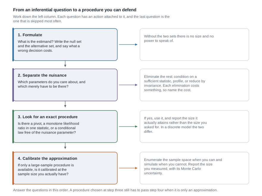
The four questions, in order

One: formulate. Write the estimand, then \(\Theta_0\) and \(\Theta_1\) as sets, then what a wrong decision costs. Until the two sets exist there is no size and no power to discuss, since both are defined by them. This step also settles whether the alternative is one-sided or two-sided, and a two-sided alternative rules Week 3’s Karlin-Rubin theorem out immediately.

Two: separate the nuisance. Which parameters are the claim, and which merely have to be in the model for it to be a model? Week 6 gave three eliminations: condition on a statistic sufficient for the nuisance parameter, profile it out, or reduce by invariance. Each costs something. Conditioning gives an exactly nuisance-free reference but discards the information in the conditioning statistic and leaves a discrete, conservative test; profiling keeps everything in view but produces a curve whose curvature overstates the precision available.

Three: look for an exact procedure. Ask whether the model hands you a pivot whose distribution is free of \(\theta\), a monotone likelihood ratio in one statistic, or a conditional law free of the nuisance parameter. If it does, the guarantee holds at every sample size. But report the size that procedure attains, not the level you asked for: in a discrete model those differ, sometimes by a factor of five.

Four: calibrate the approximation. If only a large-sample procedure is available, its claimed level is a limit statement, and a limit statement is not a promise about your \(n\). Enumerate the sample space when the model is discrete and small enough, simulate when it is not.

Reading a testing argument for what it assumes

Most flawed analyses you will meet are not wrong at any step you can point to. They are correct derivations whose first line quietly assumed something the data do not satisfy. The checklist is short: does the support of the density depend on the parameter; is the null value interior to the parameter space, and the maximizer interior too; is the model’s dimension fixed as \(n\) grows; are the expected counts large enough for a continuous reference; and has a nuisance parameter been eliminated, or merely replaced by an estimate and then forgotten?

Eight procedures from the first half, with the condition each needs and the way each breaks.

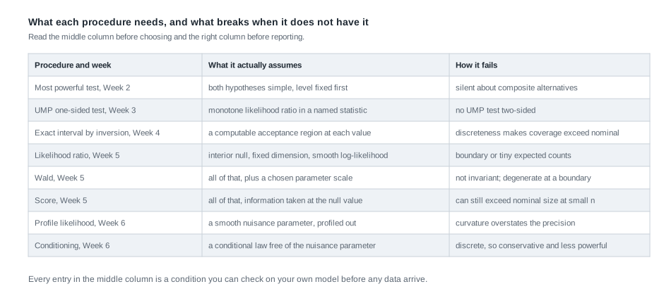
The middle column is the useful one, because every entry in it is checkable on the model before any data arrive; the right-hand column is what you owe a reader in the discussion. The eight failure modes reduce to three recurring causes: a parameter or an estimate sitting on a boundary, a discrete sample space that cannot supply the level you asked for, and a quadratic approximation asked to work where the log-likelihood is not close to quadratic. Every failure in the two worked examples below is one of those three.

Calibration as an experiment you can run

A calibration study asks one question with a numerical result: if the null hypothesis were true, how often would this procedure reject? That is the size, which Week 2 defined and every week since has assumed you could evaluate. In a discrete model you can evaluate it exactly: compute the statistic everywhere in the sample space, decide which outcomes the test rejects, and add their null probabilities. When enumeration is impossible, simulate — and the estimate then carries its own uncertainty, which you must report and must not confuse with the thing you are estimating.

Designing a size study you can defend

A size study needs four declared ingredients: the model, the null value, the nominal level, and the range of sample sizes. Let \(X \sim \text{Binomial}(n, \theta)\), test \(H_0 : \theta = 0.10\) against \(H_1 : \theta \ne 0.10\) at nominal level 0.05, and vary \(n\) from 10 to 120. Three procedures compete: the equal-tailed exact test, which rejects when the observed count lies in a tail of null probability at most \(\alpha/2\), and the likelihood-ratio and score chi-square tests of Week 5.

Attained size against sample size for an exact test and two chi-square tests.

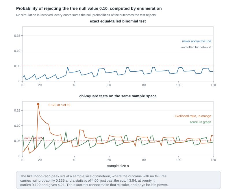
Read three things off it. The exact test never rises above the nominal line — that is the guarantee, and it holds because each tail contributes at most \(\alpha/2\) by construction. It also spends most of its time far below the line, at 0.011 when \(n = 20\) and 0.023 when \(n = 80\), the cost of exactness in a discrete model. The score curve crosses above 0.05 repeatedly, reaching 0.057 at \(n = 40\) and 0.064 at \(n = 100\); it is a good approximation, not a level-0.05 procedure. And the likelihood-ratio peak, 0.170 at \(n = 19\) with 0.133 immediately beside it at \(n = 20\), has nothing to do with small samples in general. It is one outcome: at \(n = 20\), with no failures the maximizer sits at \(\hat\theta = 0\) and \(\Lambda = 2 \times 20 \times \log(1/0.9) = 4.21\), just past the cutoff 3.84, while that outcome carries null probability 0.122. A single boundary outcome holding an eighth of the null probability does most of the damage. At \(n = 19\) that same outcome carries \(0.9^{19} = 0.135\) with statistic \(2 \times 19 \times \log(1/0.9) = 4.00\), and the upper tail, led by the count \(x = 5\) whose statistic 4.08 barely clears the cutoff, supplies the remaining 0.035.

The enumeration is a few lines of R, worth writing once so that you trust it.

attained_size <- function(n, p0, alpha = 0.05) {
  x     <- 0:n
  pmf   <- dbinom(x, n, p0)
  hat   <- x / n
  lr    <- 2 * (ifelse(x > 0, x * log(hat / p0), 0) +
                ifelse(x < n, (n - x) * log((1 - hat) / (1 - p0)), 0))
  lower <- pbinom(x, n, p0)
  upper <- 1 - pbinom(x - 1, n, p0)
  cut   <- qchisq(1 - alpha, df = 1)
  c(exact = sum(pmf[lower <= alpha / 2 | upper <= alpha / 2]),
    lr    = sum(pmf[lr > cut]))
}
attained_size(20, 0.10)

Monte Carlo error and how many replicates

When you must simulate, every point on your size curve is an estimated proportion from \(B\) independent replicates, so \(\hat p\) has standard error \(\sqrt{p(1-p)/B}\) and an approximate 95 percent interval of half-width \(1.96\sqrt{\hat p (1 - \hat p)/B}\). That is the simulation error, and more replicates shrink it. It is not the approximation error, the gap between attained size and nominal level, which no number of replicates touches. Confusing the two is the commonest defect in a simulation report: a size estimated as 0.124 with a half-width of 0.005 is not “close to 0.05 within simulation error”, it is decisively different from 0.05.

Half-width of a simulated rejection probability against the number of replicates.

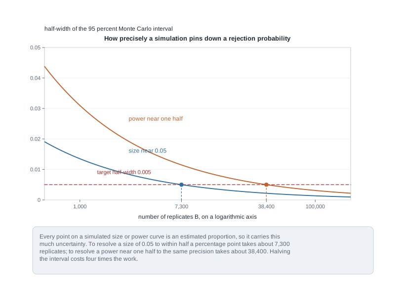
Do the arithmetic once and you stop guessing. To resolve a size near 0.05 to within half a percentage point you need \(B = (1.96)^2 (0.05)(0.95)/(0.005)^2 \approx 7{,}300\) replicates; for a power near one half at the same precision, \((1.96)^2(0.25)/(0.005)^2 \approx 38{,}400\), since the variance of a proportion is largest at one half. Halving the interval costs four times the work, so decide the precision you need before choosing \(B\).

set.seed(2027)
wald_size <- function(n, p0, B = 20000, alpha = 0.05) {
  hat  <- rbinom(B, n, p0) / n
  stat <- n * (hat - p0)^2 / (hat * (1 - hat))   # infinite when hat lands on a boundary
  phat <- mean(stat > qchisq(1 - alpha, df = 1))
  c(size = phat, mc_se = sqrt(phat * (1 - phat) / B))
}
wald_size(20, 0.10)

Comparing power only when you know the size

Power comparisons between procedures of different attained size are not comparisons. A test that rejects too often under the null rejects more often under the alternative too, and calling that an advantage is circular. Fix \(n = 20\) and the null value 0.10, and look at all three at once.

Power curves at twenty observations, with each test’s attained size marked at the null value.

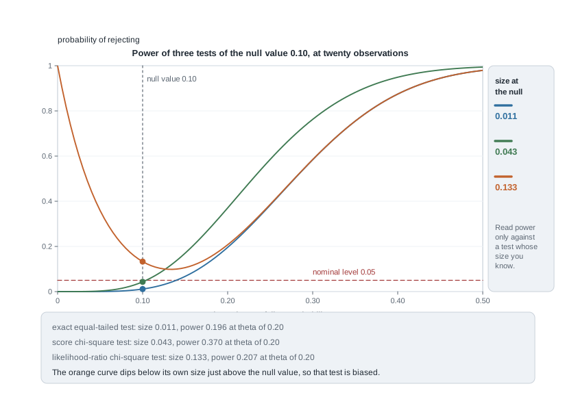
At \(\theta = 0.20\) the exact test has power 0.196 and the score test 0.370, so the score test looks nearly twice as good. Part of that is real and part is bought: the attained sizes are 0.011 and 0.043. Since both are at or below the nominal 0.05, the score test is genuinely the better buy at this \(n\) and this null value — but that sentence needed both numbers, and it does not extend to the sample sizes where the score curve sat above the line. The likelihood-ratio curve makes the point from the other side: its power at \(\theta = 0.15\) is 0.106, below its own size of 0.133, so rejecting is less likely when the null is false than when it is true. That is the failure of unbiasedness Week 3 defined. The exact test is biased too, in the other direction, with power 0.0003 at \(\theta = 0.05\), because the lower tail of a \(\text{Binomial}(20, 0.10)\) holds no outcome rare enough to reject with.

Worked example — two treatments in a small field trial

The model and the question. Sixteen plots in a field trial are split evenly between treatments A and B, and each plot either establishes a seedling or does not. Model the counts as independent \(X \sim \text{Binomial}(8, \theta_A)\) and \(Y \sim \text{Binomial}(8, \theta_B)\), observing \(x = 6\) and \(y = 2\). The claim to test is that the treatments do not differ.

Step 1, formulate. Write both success probabilities on the log-odds scale, with \(\eta = \log\{\theta_B/(1 - \theta_B)\}\) and \(\psi = \log\{\theta_A/(1-\theta_A)\} - \eta\). Then \(\psi\) is the log odds ratio, \(\Theta_0 = \{\psi = 0\}\), and \(\Theta_1 = \{\psi \ne 0\}\). The baseline \(\eta\) is a genuine nuisance parameter: unknown, not the claim, free to be anything real.

Step 2, separate the nuisance. The joint probability factors as a two-parameter exponential family,

\[ P(X = x, Y = y) = \binom{8}{x}\binom{8}{y} \frac{\exp\{\psi x + \eta t\}}{(1 + e^{\psi + \eta})^{8}(1 + e^{\eta})^{8}}, \qquad t = x + y , \]

so \(T = X + Y\) is sufficient for \(\eta\) at each fixed \(\psi\). Conditioning on \(T = t\) therefore removes \(\eta\) exactly, and the conditional law of \(X\) depends on \(\psi\) alone. This is Week 6’s conditioning route, exact rather than asymptotic. Here \(t = 8\), and at \(\psi = 0\) the conditional law is hypergeometric: \(P(X = x \mid T = 8) = \binom{8}{x}\binom{8}{8-x} / \binom{16}{8}\), with \(\binom{16}{8} = 12870\).

Step 3, choose. The exact conditional test uses the hypergeometric reference and is valid at every sample size and every value of \(\eta\), because it is valid conditionally at every \(t\). The chi-square test uses a continuous reference justified by a limit, and with expected counts of \(8 \times 8/16 = 4\) in every cell — below the customary threshold of five — that limit has little claim here. Take the exact route, and compute the approximation too, to see the disagreement.

Step 4, carry out the exact test. The upper tail counts \(\binom{8}{6}\binom{8}{2} + \binom{8}{7}\binom{8}{1} + \binom{8}{8}\binom{8}{0} = 28 \times 28 + 8 \times 8 + 1 = 849\), so \(P(X \ge 6 \mid T = 8) = 849/12870 = 0.0660\). Both margins are eight, so this hypergeometric law is symmetric about 4 and the two-sided p-value is \(2 \times 849/12870 = 0.132\), the doubling and equal-probability conventions agreeing exactly.

Step 5, compute the approximation you declined. Pearson’s statistic, in the equivalent form \(N(ad - bc)^2 / (r_1 r_2 c_1 c_2)\) for row totals \(r_i\) and column totals \(c_j\), is

\[ X^2 = \frac{16\,(6 \times 6 - 2 \times 2)^2}{8 \times 8 \times 8 \times 8} = \frac{16 \times 1024}{4096} = 4.00 , \]

with \(P(\chi^2_1 > 4.00) = 0.046\). Standardizing the same numerator by the hypergeometric variance \(r_1 r_2 c_1 c_2 / \{N^2(N-1)\} = 4096/3840 = 1.067\) gives \((6 - 4)^2/1.067 = 3.75\) instead, and 0.053. Three procedures, one table, p-values 0.046, 0.053, and 0.132.

Step 6, what the conclusion supports. At level 0.05 the exact conditional test does not reject. The estimated odds ratio is \((6 \times 6)/(2 \times 2) = 9\), which sounds large and is entirely compatible with no difference at this sample size. Be exact about what “does not reject” buys: this test rejects only when \(x \in \{0, 1, 7, 8\}\), so its attained conditional size is \(2 \times 65/12870 = 0.010\), one fifth of the level requested, and even if the odds ratio truly were 9 it would reject at these margins only about 35 percent of the time. The defensible sentence is that the trial is consistent with no difference and also with a substantial one, and that sixteen plots cannot separate the two — not that the treatments are alike.

The same reasoning, transferred

Keep the structure and change the family. Two production lines are monitored over equal exposure and their fault counts modelled as independent \(X \sim \text{Poisson}(\mu_A)\) and \(Y \sim \text{Poisson}(\mu_B)\), with \(x = 10\) and \(y = 2\). The interest parameter is \(\rho = \mu_A/\mu_B\), the nuisance parameter the overall rate \(\mu_A + \mu_B\). The same exponential-family argument applies: \(T = X + Y\) is sufficient for the total rate, and given \(T = t\) the count \(X\) is \(\text{Binomial}(t, \mu_A/(\mu_A + \mu_B))\), which under \(H_0 : \rho = 1\) is \(\text{Binomial}(12, 0.5)\) — free of the nuisance parameter, exactly.

The two-sided exact p-value counts outcomes: \(2(\binom{12}{10} + \binom{12}{11} + \binom{12}{12})/2^{12} = 2(66 + 12 + 1)/4096 = 158/4096 = 0.039\). The score statistic in the conditional binomial model simplifies to something memorable, since with \(\hat p = x/t\),

\[ S = \frac{t(\hat p - \tfrac12)^2}{\tfrac14} = \frac{(2x - t)^2}{t} = \frac{(x - y)^2}{x + y} = \frac{64}{12} = 5.33 , \]

giving \(P(\chi^2_1 > 5.33) = 0.021\). What stayed the same: the exponential-family conditioning that eliminates the nuisance parameter exactly, the discreteness of the reference, and the direction of the error, the chi-square p-value again smaller than the exact one. What changed: the family, the conditional law — binomial here, hypergeometric there — and whether the two routes agree. Here both reject at level 0.05, so the choice between them changes nothing you report. You only know that because you computed both.

Second worked example — a flawed argument from twenty devices

The argument as received. “Twenty independent devices were put on a stress test and none failed. The maximum likelihood estimate of the failure probability is \(\hat\theta = 0/20 = 0\), with estimated standard error \(\sqrt{\hat\theta(1 - \hat\theta)/20} = 0\). The 95 percent Wald interval is therefore the single point zero, and the Wald statistic for \(H_0 : \theta = 0.10\) is \((0 - 0.10)^2/0 = \infty\), so we reject overwhelmingly and conclude the failure probability is zero.”

Every arithmetic step there is correct. The conclusion is nonsense, and the repair is a sequence of named conditions.

Repair 1, name the broken condition. Week 5’s chi-square limit needs the maximizer in the interior of \(\Theta\), so that the score vanishes there and a quadratic expansion has something to expand around. Here \(\Theta = [0, 1]\) and \(\hat\theta = 0\) is a boundary point: with no failures, \(\ell(\theta) = 20\log(1 - \theta)\) and the score \(U(\theta) = -20/(1 - \theta)\) is strictly negative throughout, so it never vanishes. The estimated variance \(\hat\theta(1 - \hat\theta)/20\) is exactly zero and the information \(I_n(\theta) = 20/\{\theta(1 - \theta)\}\) diverges as \(\theta \to 0\), so the Wald statistic has no finite value. The “\(\infty\)” is software reporting a division by zero, not evidence.

Repair 2, use a procedure whose conditions hold. Under \(H_0 : \theta = 0.10\) the count is \(\text{Binomial}(20, 0.10)\), fully specified, so the exact one-sided p-value is \(P(X \le 0) = 0.9^{20} = 0.122\). About one experiment in eight produces no failures at all under exactly the hypothesis being rejected. No approximation was needed.

Repair 3, report an interval that means something. Invert the family of exact one-sided tests, as in Week 4. The set of \(\theta\) not rejected at level 0.05 is \(\{\theta : (1 - \theta)^{20} > 0.05\}\), giving the one-sided 95 percent bound \(\theta \le 1 - 0.05^{1/20} = 0.139\): with no failures in twenty trials the failure probability is plausibly anything up to about 0.14. The familiar approximation \(3/n = 0.15\) is the rough version of the same bound, and lands close, as it should.

Repair 4, calibrate before you trust. The instinct now is to abandon the Wald statistic for the likelihood ratio. Check that too: at \(x = 0\), \(\Lambda = 2\{\ell(0) - \ell(0.10)\} = 4.21\) exceeds 3.84, so it also rejects. Enumerating the sample space at \(n = 20\) and \(\theta_0 = 0.10\) gives attained sizes of 0.011 for the exact test, 0.043 for the score test, 0.133 for the likelihood ratio, and 0.124 for the Wald test, counting the boundary outcome as the rejection the software produces. The deep problem is not the choice among statistics: the only outcome in the lower tail of a \(\text{Binomial}(20, 0.10)\) is \(x = 0\), with probability 0.122. No nonrandomized test can attain a lower-tail rejection probability of 0.025 when the smallest attainable one is 0.122, so anything rejecting downward is oversized by construction — Week 2’s achievable-size arithmetic and Week 4’s discreteness conservatism arriving together.

What this licenses. You may say that twenty trials with no failures are consistent with a failure probability up to about 0.14, and that the study cannot distinguish 0.001 from 0.10. You may not say the failure probability is zero, and you may not report the Wald result.

The misreading to avoid

The misreading this week produces sounds mature rather than naive: “the exact procedure is the correct one, so when the exact and approximate results disagree I report the exact one and move on.” The first clause is defensible. The rest hides three errors.

The first is that exactness is free. In a discrete model an exact test almost never attains the level it claims, because the sample space offers only finitely many tail probabilities and the test must take one at or below \(\alpha/2\). In the field trial, “level 0.05” delivered an attained size of 0.010, and at twenty observations the exact binomial test delivered 0.011. That roughly fivefold shortfall is power you gave up. Conservative is a guarantee, not a virtue, and Week 4 already said so about coverage.

The second is that “exact” describes the p-value rather than the guarantee. What is exact is the null distribution used, and hence the validity of the level statement. It says nothing about whether the model is right, whether the conditioning discarded information you needed, or whether the estimand is what the scientific question asked about. An exact test of the wrong hypothesis is exactly wrong.

The third is that “disagree” means one procedure erred. Procedures with different attained sizes differ on borderline data by design, not by malfunction, and what is worth reporting is not which one rejected but how far each attained size sits from its nominal level. In the two-by-two table the p-values 0.046, 0.053, and 0.132 differ because the first two use a continuous reference for a nine-outcome sample space and the third uses the sample space itself.

A smaller misreading travels alongside: that a large sample size settles the matter. Large relative to what? At \(\theta_0 = 0.10\) the approximation is governed by the smaller expected count \(n\theta_0\), so \(n = 20\) gives two expected failures and behaves like a small-sample problem however the sample size is described. In the size figure the likelihood-ratio test is worse calibrated at \(n = 20\) than at \(n = 10\), because the boundary outcome becomes a rejection only once \(2n\log(1/0.9)\) exceeds 3.84, near \(n = 19\). Calibration is not monotone in \(n\).

Practice on your own

These are for self-checking, not for submission; work them before the calibration lab.

1. The order of the questions. Write the four questions and their outcomes, two sentences each, for a one-sided test of an exponential rate from twelve lifetimes; for a test that a normal mean is zero with unknown variance at \(n = 8\); and for a test that a variance component is zero. Where does step three succeed, and where does step four decide the matter?
2. Enumerate a size. Adapt the enumeration block above to \(\theta_0 = 0.05\) and compute the attained size of the exact, score, and likelihood-ratio tests for \(n = 20, 40, 80, 160\). Predict which is worst at \(n = 40\), then say what in the sample space explains it.
3. Repair a derivation. A colleague fits a two-component mixture and refers twice the log-likelihood difference against a single component to \(\chi^2_1\). Name every condition of Week 5’s theorem that fails, say which failure is fatal, and state what you would report instead.
4. Design a simulation. How many replicates pin an attained size near 0.05 to within one percentage point with 95 percent confidence? Recompute for a power near 0.80, and explain the direction of the change from the variance of a proportion.
5. Conditioning’s price. For the two-by-two table above, compute the conditional power of the level-0.05 exact test at odds ratios 4, 9, and 25, with the margins fixed. Then say in three sentences what you would tell the investigator before the next trial of this size.

set.seed(2027)
n_for_halfwidth <- function(p, half_width, conf = 0.95) {
  z <- qnorm(1 - (1 - conf) / 2)
  ceiling(z^2 * p * (1 - p) / half_width^2)
}
n_for_halfwidth(0.05, 0.01)
n_for_halfwidth(0.80, 0.01)

Where to read more

• The large-sample results this page keeps testing against their own conditions are developed in the lecture materials for MIT OpenCourseWare 18.655 Mathematical Statistics; reread the asymptotics of maximum likelihood beside the calibration figures above.
• For a slower, example-first tour of exact binomial and two-by-two procedures, see Penn State STAT 415.
• The optional Hogg, McKean, and Craig alignment for this week is Chapters 4 through 8, taken as review rather than as new reading. That book is optional and is never required to be purchased.
• Everything computed here uses base R and the stats package only; see The R Project for Statistical Computing and Quarto.
• Course pages: the syllabus, the schedule, the resources overview, and the notes overview. The units this page consolidates are Week 2 through Week 6, and Week 4’s inversion argument is worth rereading beside repair three above.

Where this goes next

The first half studied procedures one at a time, in models small enough that the whole sample space fits on a page. Week 8 changes the setting rather than the questions: the normal linear model, where the hat matrix is an orthogonal projection, degrees of freedom are ranks of projections rather than counts of parameters, and the \(t\) and \(F\) statistics are built from that geometry instead of quoted. The four questions still apply, and step three succeeds unusually often there, because normal theory hands you exact distributions for quadratic forms — but only under conditions on idempotence and centering that deserve the suspicion you have been practising here.

After that the failures move outward: many tests at once in Week 9, validity from the design rather than the model in Week 10, approximations built by resampling in Week 11. Each will be judged by the calibration study you ran here. The notes overview lists the earlier units if you need Week 3’s unbiasedness definition or Week 6’s conditioning argument first.