Week 9 — Multiplicity, multiple comparisons, and selective inference

Where this week starts

Week 8 ended with a single \(F\) statistic testing a whole subspace at once: one decision, one level, and everything Week 2 said about size applying unchanged. But nobody stops there. The \(F\) test says the group means are not all equal, and the next question is always which pair differs; a screen measures forty biomarkers and reports the three that reached significance. Each such move turns one decision into many, and the guarantee attached to one decision does not transfer to the collection.

This week asks what happens to error control when a family of tests is analysed together, and what can be repaired. The repairs come in two kinds. Controlling the family-wise error rate demands that the probability of any false rejection in the family stay at \(\alpha\); Bonferroni and Holm meet that demand without any assumption about dependence. Controlling the false discovery rate demands only that the expected proportion of false rejections among the rejections made stay at \(\alpha\); the Benjamini-Hochberg step-up rule meets that one under a dependence condition which has to be stated rather than assumed.

A third thing happens that no correction factor fixes. Every cutoff correction assumes the family was fixed before the data arrived. When the hypothesis you report was chosen because the data looked interesting, the selection is itself random, and a guarantee that averages over repeated samples with the hypothesis held fixed no longer describes what you did. By the end of the week you should want to know, of any reported effect, how many comparisons were available and whether this one was chosen before the data were seen.

Why this matters beyond the theorem

Here is the stake in its smallest form. A laboratory screens twenty inert compounds, one independent test each, every null true, each test at level 0.05. The probability that at least one is declared active is \(1 - 0.95^{20} = 0.6415\): a procedure that is exactly right twenty times over produces a false claim about two times in three, and the report describing the one significant compound will call it a five-percent-level result.

The mirror-image failure gets missed. Correcting hard enough to hold the family-wise rate at 0.05 across forty tests pushes each cutoff so far out that real effects stop being detectable, and a study that finds nothing because it corrected for forty comparisons has also failed. What this week supplies is the vocabulary to say which error rate you control, at what cost, and under what assumption about dependence.

What you will be able to do

• Define the per-comparison, family-wise, and false discovery rates from one counting table, and say which entries are observable.
• Derive the exact family-wise rate for \(m\) independent tests, compare it with the Bonferroni bound, and price the correction in power.
• Prove that Bonferroni and Holm control the family-wise rate, naming the property of a p-value each proof needs and showing that neither needs independence.
• Carry out the Benjamini-Hochberg procedure on ordered p-values and state the dependence condition its guarantee requires.
• Distinguish a planned contrast from a data-dependent selection, and give the multiplier each requires in a stated one-way layout.
• Explain why an estimate selected for significance is biased away from zero, and compute that bias exactly in a normal model.

Terms and notation worth fixing

Symbol	What it means on this page
\(m\), \(m_0\), \(m_1\)	Hypotheses in the family, those whose null is true, those whose null is false
\(I_0\)	Index set of true nulls, so \(\lvert I_0 \rvert = m_0\); unknown in practice
\(V\), \(S\), \(R\)	False rejections, true rejections, total rejections \(R = V + S\); only \(R\) is observed
\(p_{(1)} \le \cdots \le p_{(m)}\)	The p-values sorted upward, \(H_{(i)}\) carrying \(p_{(i)}\)
valid p-value	One with \(P(p \le u) \le u\) for every \(u \in [0,1]\) under its own null
\(\mathrm{FWER}\)	Family-wise error rate \(P(V \ge 1)\), the chance of any false rejection at all
\(\mathrm{FDR}\)	False discovery rate \(E(V/R)\), the ratio being defined as \(0\) when \(R = 0\)
family	The hypotheses over which a rate is controlled; a scientific choice, not a formula

Error rates for a family of tests

Everything measured this week comes out of one table. Cross-classify the \(m\) hypotheses by truth and by decision, and every error rate in the subject is a functional of the resulting counts.

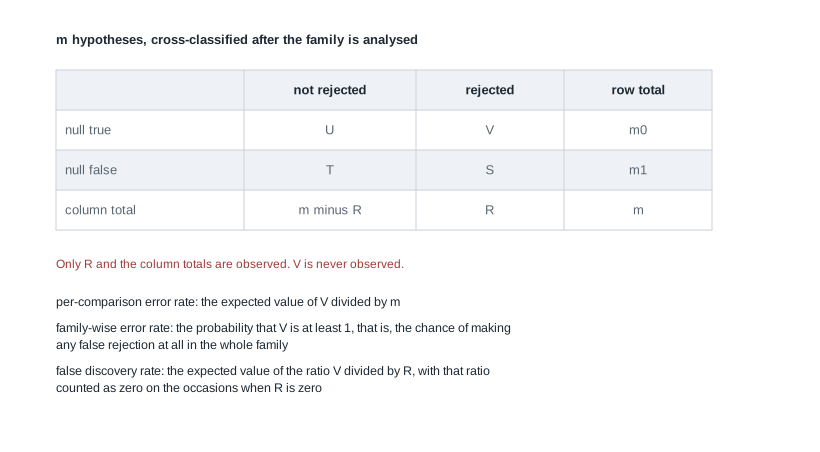
The counting table behind every multiplicity error rate, with the three rates defined from its cells.

The counting table and three error rates

Read the table as a random object: \(V\), \(S\), \(R\), \(U\), and \(T\) are statistics, while \(m_0\) and \(m_1\) are fixed unknown constants. Only \(R\) and \(m\) are ever observed, and the difficulty of the whole subject is that \(V\), the quantity every error rate is about, is invisible.

The per-comparison error rate is \(E(V)/m\). Running every test at level \(\alpha\) makes \(E(V) \le m_0 \alpha\) and so holds this rate at or below \(\alpha\), and that is all per-test control delivers. The family-wise error rate is \(\mathrm{FWER} = P(V \ge 1)\), and the false discovery rate is \(\mathrm{FDR} = E(V/R)\), with the ratio defined to be zero when \(R = 0\).

Two remarks before any procedure. The rates are ordered, since \(V/R \le \mathbf{1}\{V \ge 1\}\) pointwise, writing \(\mathbf{1}\{A\}\) for the indicator of the event \(A\): taking expectations gives \(\mathrm{FDR} \le \mathrm{FWER}\) always, so family-wise control implies false discovery control and not conversely. And the two coincide under the global null, because if every null is true then \(V = R\) and \(V/R\) is exactly \(\mathbf{1}\{R \ge 1\}\). Every false-discovery procedure therefore controls the family-wise rate in the weak sense, and only in that sense.

Now watch the family-wise rate grow. Let the \(m\) tests be independent, every null true, and each test of size exactly \(\alpha\), which is available whenever the statistic is continuous. Then \(\mathrm{FWER} = 1 - (1-\alpha)^m\), climbing from 0.05 at \(m = 1\) to 0.64 at \(m = 20\) and 0.92 at \(m = 50\).

Family-wise error rate against the number of tests, with and without a divided cutoff.

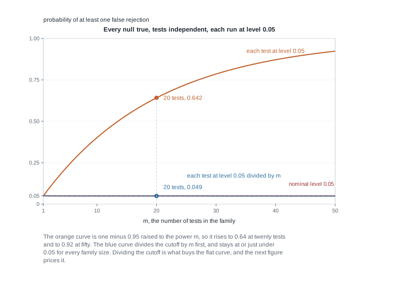
Independence is doing real work in that formula. Were the tests perfectly dependent, one statistic reported \(m\) times, the rate would stay at \(\alpha\) for every \(m\); real families sit between, so \(1 - (1-\alpha)^m\) shows how bad the problem can get rather than a universal value.

Bonferroni and Holm, and what each proof needs

The Bonferroni procedure rejects \(H_i\) when \(p_i \le \alpha/m\). Suppose each \(p_i\) with \(i \in I_0\) is valid, meaning \(P(p_i \le u) \le u\) for every \(u\) in \([0,1]\) under its own null. Then

\[ \mathrm{FWER} = P\!\left(\bigcup_{i \in I_0} \{p_i \le \alpha/m\}\right) \le \sum_{i \in I_0} P(p_i \le \alpha/m) \le m_0 \frac{\alpha}{m} \le \alpha . \]

The first inequality is Boole’s, which holds for any events at all; the second is validity of each p-value separately. No independence is used, and none is needed: a union bound never asks how the events overlap, which is why Bonferroni survives where nothing about the joint distribution is known. It also locates the conservatism: the bound settles for \(m_0\alpha/m\) rather than \(\alpha\), and gives away more still when the rejection events overlap.

Holm’s step-down procedure recovers part of that at no cost in assumptions. Sort the p-values and compare \(p_{(i)}\) with \(\alpha/(m - i + 1)\) in order from \(i = 1\); stop at the first failure and reject exactly the hypotheses before it, rejecting all \(m\) if no comparison fails. The first threshold is \(\alpha/m\), identical to Bonferroni’s, and every later one is larger, so Holm rejects everything Bonferroni does.

The proof turns on the shape of the rejection set. Suppose at least one true null is rejected, and let \(H_h\) be the one of smallest rank among the rejected true nulls, sitting at rank \(j\). Holm’s rejection set is the block carrying the smallest p-values, so every hypothesis ranked ahead of \(H_h\) is rejected too, and by the minimality of \(j\) none of those \(j - 1\) hypotheses is a true null. Hence \(j - 1 \le m - m_0\), that is \(m - j + 1 \ge m_0\), while \(H_h\) being rejected at rank \(j\) means \(p_h \le \alpha/(m - j + 1)\). Therefore

\[ V \ge 1 \quad \Longrightarrow \quad p_h \le \frac{\alpha}{m - j + 1} \le \frac{\alpha}{m_0} , \]

and \(\mathrm{FWER} \le P(\min_{i \in I_0} p_i \le \alpha/m_0) \le m_0 \cdot \alpha/m_0 = \alpha\) by Boole’s inequality again. Validity enters at that last step and independence never appears. Holm is therefore uniformly at least as powerful as Bonferroni under identical assumptions.

Controlling the false discovery rate

Family-wise control asks a lot. When a screen tests twenty thousand hypotheses expecting a few hundred real effects, insisting that the probability of even one false rejection stay at 0.05 discards nearly all the power. The false discovery rate asks instead: among the findings you announce, what fraction do you expect to be wrong?

The step-up rule and why it works

The Benjamini-Hochberg procedure at level \(\alpha\) sorts the p-values, computes

\[ \hat k = \max\{\, i \in \{1, \dots, m\} : p_{(i)} \le i\alpha/m \,\}, \]

with \(\hat k = 0\) when no index qualifies, and rejects \(H_{(1)}, \dots, H_{(\hat k)}\). Note the word max. This is a step-up rule: it scans downward from the largest p-value, stops at the first one under its own sloping threshold, and rejects that hypothesis and every hypothesis below it. A hypothesis whose own p-value sits above its own threshold is still rejected when a larger p-value clears a later one.

The theorem is due to Benjamini and Hochberg. Assume (i) each \(p_i\) with \(i \in I_0\) is valid, and (ii) the null p-values are independent of one another and of the non-null p-values. Then \(\mathrm{FDR} \le (m_0/m)\,\alpha \le \alpha\).

The derivation is short and isolates the step that needs (ii). Since \(R = \hat k\), and \(H_i\) is rejected exactly when \(p_i \le \hat k \alpha/m\),

\[ \mathrm{FDR} = \sum_{i \in I_0} E\!\left[\frac{\mathbf{1}\{p_i \le \hat k \alpha/m\}}{\hat k}\right] = \sum_{i \in I_0} \sum_{k=1}^{m} \frac{1}{k}\, P\!\left(p_i \le \frac{k\alpha}{m},\ \hat k = k\right). \]

Fix \(i\) and \(k\) and work on the event \(\{p_i \le k\alpha/m\}\). There, \(\hat k = k\) says two things about the other \(m - 1\) p-values and nothing about \(p_i\): at least \(k - 1\) of them lie at or below \(k\alpha/m\), and for each \(l > k\) fewer than \(l - 1\) of them lie at or below \(l\alpha/m\). Write \(\hat k^{(i)}\) for the index the same rule produces when \(p_i\) is replaced by zero; since zero clears every threshold, that pair of statements is exactly \(\{\hat k^{(i)} = k\}\), so

\[ \left\{p_i \le \frac{k\alpha}{m}\right\} \cap \{\hat k = k\} = \left\{p_i \le \frac{k\alpha}{m}\right\} \cap \{\hat k^{(i)} = k\} , \]

and the second event is a function of \((p_j)_{j \ne i}\) alone. This is the only place independence is used: it lets the probability factor, and validity then bounds the first factor by \(k\alpha/m\). Substituting, the \(k\) cancels and the sum collapses,

\[ \sum_{k=1}^{m} \frac{1}{k}\cdot\frac{k\alpha}{m}\,P(\hat k^{(i)} = k) = \frac{\alpha}{m}\sum_{k=1}^{m} P(\hat k^{(i)} = k) = \frac{\alpha}{m}, \]

because \(\hat k^{(i)} \ge 1\) always — setting \(p_i\) to zero guarantees the first comparison passes — so those \(m\) events partition the sample space. Summing over the \(m_0\) true nulls gives \((m_0/m)\alpha\).

Two things the derivation shows that the statement does not. The bound is \((m_0/m)\alpha\) rather than \(\alpha\), so the procedure gives away the fraction \(m_1/m\) of the level it was allowed, and methods that estimate \(m_0\) from the data recover that slack. And the guarantee bounds an expectation over repeated experiments: the realized \(V/R\) in your one data set is random and can sit far above \(\alpha\).

What the dependence condition buys

Condition (ii) is often implausible, since p-values from tests sharing a control group, a pooled variance estimate, or a common latent factor are dependent by construction. Two results describe what survives. Under positive regression dependence on each null p-value, which holds for one-sided tests on jointly normal statistics with non-negative correlations, Benjamini and Yekutieli showed the same bound \((m_0/m)\alpha\). Under arbitrary dependence the level must be divided by \(\sum_{j=1}^{m} 1/j\), about 2.93 at \(m = 10\) and about 5.19 at \(m = 100\): close to Bonferroni’s price, and the honest cost of knowing nothing about the joint distribution. The practical statement is therefore precise: Bonferroni and Holm need no dependence assumption, while Benjamini-Hochberg needs independence or positive regression dependence among the null p-values, or a divided level.

When selection chooses the hypothesis

Every correction above assumed the family was fixed in advance. Once the hypothesis you report is chosen using the data, something different has gone wrong, and no multiplier repairs it.

Planned contrasts and data-dependent selection

Take a balanced one-way layout of four groups of six, so \(N = 24\), the residual carries \(N - k = 20\) degrees of freedom, and one pooled variance estimate is shared by every comparison. A planned contrast is a fixed vector \(c\) with \(\sum_j c_j = 0\), specified before the data arrive; for it, \(\sum_j c_j \bar Y_j\) over its estimated standard error has an exact \(t\) distribution on 20 degrees of freedom, and the two-sided multiplier is the 0.975 quantile 2.086. The contrasts you might have chosen instead never enter.

Look instead at the six pairwise differences and discuss the largest, and what you are reporting is a maximum of six dependent quantities, with no \(t\) distribution. Three standard repairs give three multipliers for this one design:

• Tukey, exact for all six pairwise differences at once, uses the studentized range: \(q_{0.05}(4, 20)/\sqrt{2} = 3.958/\sqrt{2} = 2.80\), with \(q_{0.05}(4, 20)\) the level-0.05 critical value of the studentized range of four means on 20 degrees of freedom.
• Bonferroni over the six comparisons uses the \(t\) quantile at \(1 - 0.05/12\), namely 2.93.
• Scheffé, valid simultaneously for every contrast, including one chosen after seeing the data, uses \(\sqrt{(k-1)F_{0.95}(3, 20)} = \sqrt{3 \times 3.098} = 3.05\), with \(F_{0.95}(3, 20) = 3.098\) the 0.95 quantile of the \(F\) law on 3 and 20 degrees of freedom.

The ordering \(2.09 < 2.80 < 2.93 < 3.05\) is a price list for how much freedom you reserved, and it explains Scheffé’s expense: that method alone protects a contrast chosen after looking.

The guarantee selective inference asks for

Selection damages more than the p-value. Let \(\hat\theta_j \sim N(\theta_j, 1)\) independently, in units where the standard error is one, and report an effect only when \(\hat\theta_j > 1.96\). For a coordinate with \(\theta_j = 0\),

\[ E(\hat\theta_j \mid \hat\theta_j > 1.96) = \frac{\varphi_{\mathrm{N}}(1.96)}{1 - \Phi(1.96)} = \frac{0.0584}{0.0250} = 2.34 , \]

writing \(\varphi_{\mathrm{N}}\) and \(\Phi\) for the standard normal density and distribution function. The estimator is exactly unbiased before selection and biased by 2.34 standard errors after it. This is the winner’s curse, and it is worst where the true effect is small.

Reported effects against the true effects that generated them, after selecting for significance.

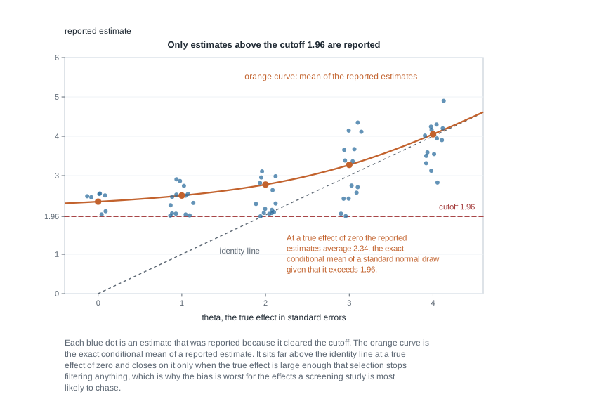
The interval fails too, and totally rather than partially. The usual \(\hat\theta_j \pm 1.96\) has coverage 0.95 for every \(\theta_j\) unconditionally, but conditional on the selection event \(\hat\theta_j > 1.96\) the whole interval lies above zero, so its conditional coverage of the value \(\theta_j = 0\) is exactly zero. Nothing unconditional was false; it simply does not describe the intervals you chose to print.

Selective inference restores a guarantee conditional on the selection event, and two ideas suffice here. One computes the conditional law directly: given \(\hat\theta_j > c\) the estimate is truncated normal, and inverting tests built on that law yields an interval with conditional coverage \(1 - \alpha\), wider and pulled toward zero. The other is sample splitting: choose the hypotheses on one half of the data and test them on the other, so the selection event is independent of the second half and the ordinary guarantee applies unchanged, at the cost of half the data for each job.

Worked example — twenty independent tests with every null true

The model and the question. Twenty candidate compounds are screened, one independent assay each. Assay \(j\) yields \(Z_j \sim N(\theta_j, 1)\), in units where the standard error is one, and the test of \(H_{0j} : \theta_j = 0\) against a two-sided alternative rejects when \(p_j \le 0.05\), that is when \(\lvert Z_j \rvert\) exceeds the 0.975 standard normal quantile, 1.96 to two decimals. Because \(Z_j\) is continuous, that test has size exactly 0.05. Take the case where every compound is inert, so \(\theta_j = 0\) and \(m_0 = m = 20\).

Step 1, the exact family-wise rate. The tests are independent, so the twenty non-rejection events are independent and

\[ \mathrm{FWER} = 1 - (1 - 0.05)^{20} = 1 - 0.3585 = 0.6415 . \]

Step 2, the expected number of false rejections. \(V \sim \mathrm{Binomial}(20, 0.05)\), so \(E(V) = 1\) exactly: on average this screen manufactures one spurious active compound per run.

Step 3, Bonferroni and its exact size. Reject only when \(p_j \le 0.05/20 = 0.0025\). With independent tests each of size exactly 0.0025, the exact family-wise rate is \(1 - (1 - 0.0025)^{20} = 0.04883\), just under 0.05. The shortfall of about 0.0012 is the conservatism the union bound left behind, small here because \(m_0/m = 1\) and the events barely overlap at such small probabilities. Under independence the exactly calibrated cutoff is Šidák’s, \(1 - 0.95^{1/20} = 0.002561\), marginally larger — but that calculation breaks under dependence and Bonferroni’s bound does not.

Step 4, the cost in power. A two-sided test at level 0.0025 rejects when \(\lvert Z_j \rvert \ge 3.023\), the 0.99875 quantile of the standard normal, against 1.96 before. For a compound genuinely active at \(\theta_j = 3\), power was \(\Phi(3 - 1.96) = \Phi(1.04) = 0.851\), ignoring the negligible opposite tail, and after correction it is \(\Phi(3 - 3.023) = \Phi(-0.023) = 0.491\).

Power of one two-sided test after the level is divided among m tests, at two effect sizes.

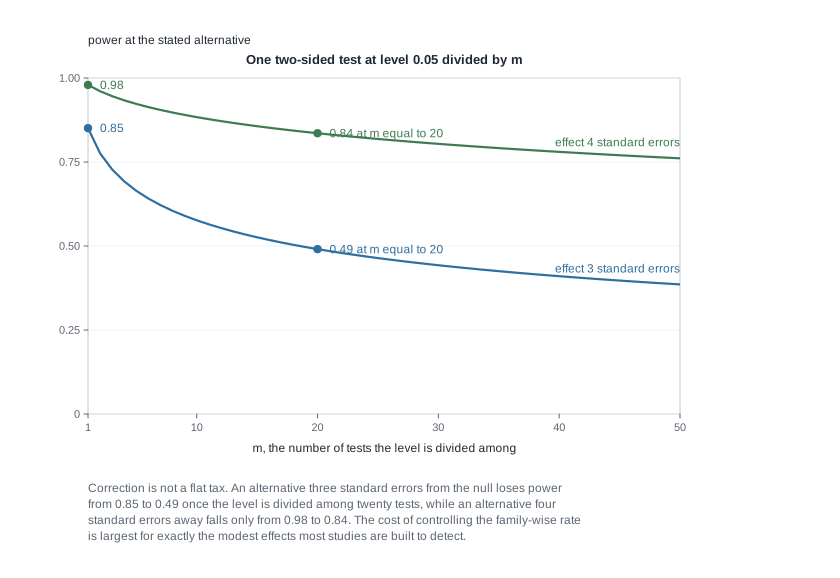
Step 5, whom the correction hurts. The figure repeats the calculation at an effect of four standard errors, where power falls only from 0.979 to 0.836. Family-wise control is not a flat tax: its cost concentrates on the modest effects a screening study is built to find.

What this licenses. You may say that an uncorrected screen of twenty independent tests has probability 0.6415 of at least one false positive, and that Bonferroni brings that to 0.0488 at a power cost of about 0.36 here. You may not carry 0.6415 to a screen whose tests are dependent, since that number came from the independence used in step 1.

m <- 20; alpha <- 0.05
1 - (1 - alpha)^m                       # exact family-wise rate, independent tests
1 - (1 - alpha / m)^m                   # exact rate after the Bonferroni cutoff
1 - (1 - alpha)^(1 / m)                 # the Sidak cutoff, exact under independence
pnorm(3 - qnorm(1 - alpha / 2))         # power at an effect of 3, uncorrected
pnorm(3 - qnorm(1 - alpha / (2 * m)))   # power at an effect of 3, corrected

The same reasoning, transferred

Change the family and keep the reasoning. Return to the balanced layout of four groups of six above, with its twenty residual degrees of freedom, and the six pairwise comparisons among the group means.

What stays the same is the union bound, and therefore Bonferroni: comparing each pairwise p-value with \(0.05/6 = 0.00833\), equivalently using the multiplier 2.93, controls the family-wise rate at or below 0.05 with no assumption about how the six comparisons depend on one another. Holm applies verbatim, with thresholds \(0.05/6, \dots, 0.05/1\) in order.

What changes is that step 1’s exact calculation is unavailable. The six \(t\) statistics share one pooled variance estimate, and each group mean appears in three of them, so they are dependent, and \(1 - 0.95^6 = 0.2649\) is not the uncorrected family-wise rate: it is what that rate would be were the six tests independent, which they are not. Exploiting the dependence beats ignoring it, since Tukey’s multiplier 2.80 attains family-wise rate exactly 0.05 in this balanced design where Bonferroni’s 2.93 only bounds it. Bounds survive dependence; exact calculations do not.

Second worked example — a step-up rule on ten ordered p-values

The setting. Ten hypotheses fixed in advance are tested, one p-value each, ordered:

\[ 0.0008,\ 0.0090,\ 0.0120,\ 0.0190,\ 0.0260,\ 0.0295,\ 0.2100,\ 0.3500,\ 0.6300,\ 0.8900 . \]

Apply Bonferroni, Holm, and Benjamini-Hochberg at \(\alpha = 0.05\), and compare.

Step 1, Bonferroni. The cutoff is \(0.05/10 = 0.005\); only \(p_{(1)} = 0.0008\) falls below it, so one hypothesis is rejected.

Step 2, Holm. Compare \(p_{(i)}\) with \(0.05/(11-i)\) in order. At \(i = 1\), \(0.0008 \le 0.0050\), so reject. At \(i = 2\), \(0.0090\) against \(0.05/9 = 0.00556\): the comparison fails and Holm stops, having rejected one.

Step 3, Benjamini-Hochberg as a step-up. The sloping thresholds are \(i \times 0.005\). From the top: \(0.8900 > 0.050\), \(0.6300 > 0.045\), \(0.3500 > 0.040\), \(0.2100 > 0.035\), and then \(0.0295 \le 0.030\) — a crossing at \(i = 6\). So \(\hat k = 6\) and the six smallest p-values are rejected.

Ten ordered p-values against the Bonferroni and Benjamini-Hochberg cutoffs, whole and magnified.

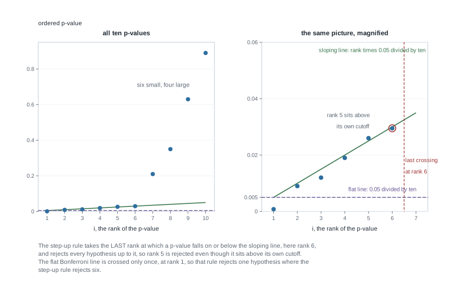
Step 4, the step-up feature. Rank 5 carries p-value 0.0260, above its own threshold \(5 \times 0.005 = 0.025\), and is rejected anyway. That is what max in the definition of \(\hat k\) requires, since a later crossing pulls every earlier hypothesis in with it. Run these same sloping thresholds downward instead, in Holm’s manner, and you stop at the first failure — rank 5 — and reject only four.

Step 5, adjusted values as a cross-check. The adjusted value at rank \(i\) is \(\min_{j \ge i}\min(1, m\,p_{(j)}/j)\), a running minimum from the largest rank downward. The raw ratios \(m\,p_{(j)}/j\) are \(0.0080\), \(0.0450\), \(0.0400\), \(0.0475\), \(0.0520\), \(0.0492\), \(0.3000\), \(0.4375\), \(0.7000\), \(0.8900\), and the running minimum makes them monotone:

\[ 0.0080,\ 0.0400,\ 0.0400,\ 0.0475,\ 0.0492,\ 0.0492,\ 0.3000,\ 0.4375,\ 0.7000,\ 0.8900 . \]

Exactly six are at or below 0.05, agreeing with \(\hat k = 6\). At rank 5 the own ratio 0.0520 exceeds 0.05, and the value borrowed from rank 6 brings it to 0.0492: monotonicity enforcement and the step-up rule are one device seen twice.

Step 6, if the dependence is unknown. Divide the level by \(\sum_{j=1}^{10} 1/j = 2.929\), giving \(0.05/2.929 = 0.01707\) and thresholds \(i \times 0.001707\). Only rank 1 clears, so under arbitrary dependence the procedure rejects one hypothesis, the same as Bonferroni on this list. The step-up rule’s whole advantage here rested on the dependence condition being defensible.

What this licenses. With independence or positive regression dependence among the null p-values, you may say that the procedure which produced these six findings has false discovery rate at most 0.05, and in fact at most \((m_0/10)(0.05)\). You may not say that any one of the six has a 5 percent chance of being wrong, nor that the realized error proportion is at most 0.05 here: \(V/6\) is random, 0.05 bounds only its average over repetitions, and that average is not taken holding \(R\) at six.

p <- c(0.0008, 0.0090, 0.0120, 0.0190, 0.0260, 0.0295, 0.21, 0.35, 0.63, 0.89)
round(p.adjust(p, method = "BH"), 4)
round(p.adjust(p, method = "holm"), 4)
c(bh = sum(p.adjust(p, "BH") <= 0.05), holm = sum(p.adjust(p, "holm") <= 0.05))

The misreading to avoid

The misreading arrives confidently: “I controlled the false discovery rate at 5 percent, so each of my six findings has at most a 5 percent chance of being wrong.” It sounds like the careful version of a claim, and it is a different claim from the theorem’s.

The false discovery rate is \(E(V/R)\), an average over hypothetical repetitions of a ratio of counts. It is a property of the procedure, not of any one rejection, and it says nothing about which finding is the false one. Nor does it constrain the realized proportion: in the second worked example \(V/6\) could be \(0\), \(1/6\), or \(1\), and the guarantee bounds only its average, with wide spread when \(R\) is small. The quantity that does answer “is this finding wrong” is a posterior probability, which needs a prior on which nulls are true.

Two smaller misreadings travel with the big one. The first is that a correction repairs selection. It does not: all three procedures assume the family was fixed before the data were seen, and they adjust cutoffs rather than the fact that you chose what to look at. Examine forty subgroups, pick the striking one, and apply a factor of forty, and you have done something defensible; report it uncorrected because it was “the obvious comparison”, and the correction you owe is invisible while the estimate still carries the selection bias computed above.

The second is that the family is determined by the mathematics. Nothing in any theorem here tells you whether the family is one table, one paper, or one set of primary endpoints fixed in advance. That is a scientific judgement, it fixes \(m\) and therefore every cutoff, and the defensible practice is to state the family you chose, and why, before the data are examined.

Practice on your own

These are for self-checking; work them before the calibration lab rather than after.

1. The exact rate under dependence. Two statistics are bivariate normal with correlation \(\rho\), each tested two-sided at level 0.05 under a true null. Estimate the family-wise rate by simulation for \(\rho = 0, 0.5, 0.9, 1\), check the extremes against \(1 - 0.95^2\) and \(0.05\), and confirm the Bonferroni cutoff holds the rate at or below 0.05 for every \(\rho\).
2. Holm strictly beats Bonferroni. Construct a list of five p-values on which Holm rejects strictly more hypotheses than Bonferroni at \(\alpha = 0.05\), and a second on which the two agree. Say in one sentence what property of the list decides it.
3. Where the step-up rule bites. Take the ten p-values above and change \(p_{(6)}\) from 0.0295 to 0.0305, leaving the rest fixed. Recompute \(\hat k\) and the adjusted values, and explain why a change of 0.001 in one p-value changes the number of rejections by two.
4. A simulation of both rates. Simulate families of \(m = 100\) tests with \(m_0 = 90\) true nulls and ten alternatives at an effect of three standard errors. Over two thousand replicates estimate the family-wise and false discovery rates of the uncorrected, Bonferroni, Holm, and Benjamini-Hochberg procedures, report the mean number of true rejections each achieves, and give each estimate’s Monte Carlo standard error.
5. Selection bias, derived. For \(\hat\theta \sim N(\theta, 1)\) reported only when \(\hat\theta > c\), derive \(E(\hat\theta \mid \hat\theta > c) = \theta + \varphi_{\mathrm{N}}(c-\theta)/\{1 - \Phi(c-\theta)\}\), verify 2.34 at \(\theta = 0\) and \(c = 1.96\), and show the bias tends to zero as \(\theta\) grows.

set.seed(2027)
one_family <- function(m0, m1, effect, alpha = 0.05) {
  z <- c(rnorm(m0), rnorm(m1, mean = effect))
  p <- 2 * pnorm(abs(z), lower.tail = FALSE)
  rejected <- p.adjust(p, method = "BH") <= alpha
  c(false_rejections = sum(rejected[seq_len(m0)]), total = sum(rejected))
}
out <- replicate(2000, one_family(90, 10, 3))
mean(out["false_rejections", ] >= 1)
mean(ifelse(out["total", ] > 0, out["false_rejections", ] / out["total", ], 0))

Where to read more

• The decision-theoretic framing of simultaneous inference is developed in the lecture materials for MIT OpenCourseWare 18.655 Mathematical Statistics.
• A slower, example-first treatment of multiple comparisons following an analysis of variance, useful if the Tukey and Scheffé multipliers went past quickly, is in Penn State STAT 415.
• The optional Hogg, McKean, and Craig alignment for this week is Chapter 9.2 together with Chapter 9.4 through 9.6. That book is optional and is never required to be purchased.
• Every computation here runs in base R with the stats package, whose p.adjust implements all four corrections used above; see The R Project for Statistical Computing and Quarto.
• Course pages: the syllabus, the schedule, the resources overview, and the notes overview. The projection geometry behind any one-way layout is developed in Week 8.

Where this goes next

Every correction here took the p-values as given and adjusted the cutoffs, which leaves open where a trustworthy p-value comes from when the model is doubtful. Week 10 answers that from a different direction: a randomization or permutation test is valid because the randomization actually happened, not because a distributional assumption held. Two threads continue there. A permutation test gives an exact null distribution for one comparison, so it repairs calibration but not multiplicity, and you will still need the machinery above when it is run on forty outcomes. And conditioning reappears as the argument behind exact tests, eliminating a nuisance parameter rather than a selection event.

If a step went past you, repair the Bonferroni proof first, since Holm’s argument is the same union bound on a smaller set, and the step-up definition second, because the max is where nearly every hand-worked mistake happens. The notes overview lists the earlier units of the course.