Week 6 — Nuisance parameters, profiling, and local alternatives
Where this week starts
Week 5 built three statistics from one log-likelihood and gave you one limiting distribution to refer them to. Every calculation there carried a convenience almost no real problem grants: the null pinned down the entire parameter, so the log-likelihood was a curve over one axis and the drop from its maximum to the null value was unambiguous.
Take one step toward the models you will actually fit and that convenience is gone. You care whether a mean equals a stated value but do not know the variance; you care about a treatment effect but not about the baseline rate it acts on. The parameter splits as \(\theta = (\psi, \lambda)\): the interest parameter \(\psi\) carries the scientific claim, the nuisance parameter \(\lambda\) holds everything else the model needs in order to be a model, and a hypothesis about \(\psi\) alone names a slice of a surface rather than a point.
This week develops the three honest routes from that surface back to a curve over \(\psi\) — maximize the nuisance out, condition on a statistic that carries it, or reduce the problem by a group of transformations that leaves it unchanged — and what each route costs. The second half answers a question the first raises: against a fixed alternative every consistent test has power tending to one, so asymptotic comparisons collapse into a tie, and local alternatives are what keep them alive. What should feel different by the end is your reaction to a profile likelihood plot: it looks exactly like a log-likelihood, and treating it as one is the error this material most reliably produces.
Why this matters beyond the theorem
Here is the stake in the smallest example this page can offer. A clinical laboratory measures ten specimens and reports a sample mean of 4.80 with a total squared deviation about that mean of 3.20; the question is whether the underlying mean is 4.40. Someone profiles the unknown variance out of the normal likelihood, takes twice the drop from the maximum to the null value, gets 4.055, compares it with 3.84, and reports a significant departure at the 0.05 level. The exact procedure here is the ordinary \(t\) test, and it gives 0.063. No arithmetic error was made: a profile log-likelihood was treated as a genuine one, and the reference distribution belonging to a genuine one was used.
The failure runs the other way when the nuisance parameter is discrete. A field trial compares two groups of seven units and sees five successes in one and one in the other. A chi-square test on that table returns 0.031; an exact test conditioning on the observed margins, which cancels the unknown baseline rate entirely, returns 0.103. Which elimination you trust is not a technicality here; it is the inference.
What you will be able to do
- Construct the profile log-likelihood for a two-parameter model and derive its curvature at the maximum as the appropriate block of the inverse observed information.
- State the conditions under which the profile likelihood-ratio statistic has a chi-square limit, and name the one that fails when the nuisance dimension grows with the sample.
- Explain why a profile likelihood is not a likelihood, quantify the overstatement of precision that follows, and name the corrections that exist.
- Eliminate a nuisance parameter by conditioning or by invariance, saying what the reduction buys and what it discards.
- Compute the effective information beside a correlated nuisance parameter, and convert the loss into lost power or an inflated sample size.
- Define a sequence of local alternatives, give the noncentrality of the limiting distribution, and explain why the three classical tests share one limiting power function while disagreeing at every finite sample size.
Terms and notation worth fixing
| Symbol | What it means on this page |
|---|---|
| \(\psi\), \(\lambda\) | The interest parameter and the nuisance parameter, with \(\theta = (\psi, \lambda)\) |
| \(\hat\lambda_\psi\) | The value of \(\lambda\) maximizing \(\ell(\psi, \lambda)\) with \(\psi\) held fixed |
| \(\ell_P(\psi)\) | The profile log-likelihood \(\ell(\psi, \hat\lambda_\psi)\), a curve over \(\psi\) alone |
| \(J(\theta)\) | Observed information, with blocks \(J_{\psi\psi}\), \(J_{\psi\lambda}\), \(J_{\lambda\lambda}\) |
| \(i(\theta)\) | Expected information for one observation, so the sample information is \(n\,i(\theta)\) |
| \(i_{\psi\psi \cdot \lambda}\) | Effective information \(i_{\psi\psi} - i_{\psi\lambda} i_{\lambda\lambda}^{-1} i_{\lambda\psi}\), what is left about \(\psi\) once \(\lambda\) is eliminated |
| \(\psi_n = \psi_0 + h/\sqrt{n}\) | A local alternative with drift \(h\), approaching the null as the sample grows |
| \(\chi^2_q(\nu)\) | Noncentral chi-square on \(q\) degrees of freedom with noncentrality \(\nu\); at \(\nu = 0\) the ordinary \(\chi^2_q\) |
Profiling a nuisance parameter away
Fix a model \(\{f(\cdot\,; \psi, \lambda)\}\) with \(\psi\) of dimension \(q\) and \(\lambda\) of dimension \(p - q\), both ranging over open sets. The profile log-likelihood is
\[ \ell_P(\psi) = \max_{\lambda} \ell(\psi, \lambda) = \ell(\psi, \hat\lambda_\psi), \]
where \(\hat\lambda_\psi\) maximizes \(\ell\) over \(\lambda\) with \(\psi\) held fixed. Hold the geometry in mind before any algebra: the two-parameter log-likelihood is a surface, \(\hat\lambda_\psi\) traces a ridge across it, and \(\ell_P\) is the height along that ridge. Its competitor is the slice you would draw if the nuisance parameter were known and equal to its estimate.
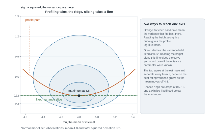
The two agree at the overall maximum, where \(\hat\lambda_{\hat\psi} = \hat\lambda\), and separate as \(\psi\) moves away. In the picture the ridge climbs, because a mean far from the sample mean forces a larger fitted variance to accommodate the same data.
The profile likelihood and its curvature
Both facts we need come from differentiating the equation defining \(\hat\lambda_\psi\), namely \(\ell_\lambda(\psi, \hat\lambda_\psi) = 0\), where a subscript denotes a partial derivative. Differentiating in \(\psi\) gives \(\ell_{\lambda\psi} + \ell_{\lambda\lambda}\,\partial \hat\lambda_\psi / \partial \psi = 0\), so \(\partial \hat\lambda_\psi / \partial \psi = -\ell_{\lambda\lambda}^{-1} \ell_{\lambda\psi}\), which requires \(\ell_{\lambda\lambda}\) to be nonsingular there — the first place a condition enters. Now differentiate \(\ell_P\). Because \(\ell\) is stationary in \(\lambda\) at \(\hat\lambda_\psi\), the chain-rule term drops out, leaving the envelope identity \(\ell_P'(\psi) = \ell_\psi(\psi, \hat\lambda_\psi)\): the profile score is the \(\psi\) component of the ordinary score, read along the ridge. Differentiating once more, keeping that term,
\[ \ell_P''(\psi) = \ell_{\psi\psi} + \ell_{\psi\lambda}\frac{\partial \hat\lambda_\psi}{\partial \psi} = \ell_{\psi\psi} - \ell_{\psi\lambda}\,\ell_{\lambda\lambda}^{-1}\,\ell_{\lambda\psi}, \qquad\text{so}\qquad -\ell_P''(\hat\psi) = J_{\psi\psi} - J_{\psi\lambda} J_{\lambda\lambda}^{-1} J_{\lambda\psi}. \]
The right-hand side is the whole story of what profiling does. It is a Schur complement, equal to the inverse of the \(\psi\) block of \(J^{-1}\): the curvature of the profile at its maximum is exactly the precision the joint fit attaches to \(\hat\psi\), with the uncertainty in \(\hat\lambda\) already discounted. It is never larger than \(J_{\psi\psi}\), the curvature you would have had with \(\lambda\) known, and the gap is the first-order cost of the nuisance parameter.
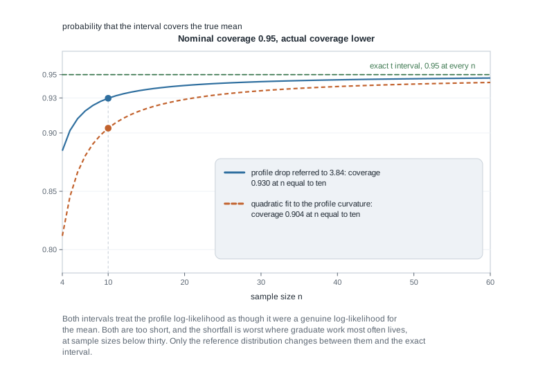
So the profile is not naive. Why is it still not a likelihood? Because being a likelihood is a distributional claim, not a shape. A genuine log-likelihood satisfies two identities: its score has mean exactly zero, and the variance of that score equals the expected information. Neither holds exactly for \(\ell_P\), and the discrepancies are of order one — negligible beside a score of order \(\sqrt{n}\) and an information of order \(n\), which is why a chi-square limit survives, but not negligible at \(n = 10\). The symptom appears below: the profile curvature there is the known-variance information with the variance replaced by its maximum likelihood estimate, which is biased low, so the curvature runs too large and the interval too short.
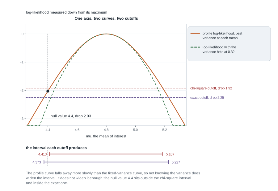
Under conditions matching Week 5’s, with \(\psi_0\) interior, the nuisance parameter of fixed dimension and estimable at rate \(\sqrt{n}\), and \(i(\theta)\) positive definite at the truth, \(\Lambda_P = 2\{\ell_P(\hat\psi) - \ell_P(\psi_0)\}\) converges in distribution to \(\chi^2_q\) under the null. That licenses the usual practice, not the belief that the approximation is good at your sample size, and the figure above is a case where it is not.
Parameter orthogonality and the information you lose
Take expectations in the curvature identity and the same Schur complement reappears with \(i\) in place of \(J\). The effective information for \(\psi\) is \(i_{\psi\psi \cdot \lambda} = i_{\psi\psi} - i_{\psi\lambda} i_{\lambda\lambda}^{-1} i_{\lambda\psi}\), and the asymptotic variance of \(\hat\psi\) is \((n\, i_{\psi\psi \cdot \lambda})^{-1}\). Two parameters are orthogonal at \(\theta\) when \(i_{\psi\lambda} = 0\) there, which is exactly when the correction vanishes and the nuisance parameter costs no information at first order.
The geometry says it better than the algebra. A confidence region for \((\psi, \lambda)\) is an ellipse. Profiling reads off its shadow on the \(\psi\) axis; slicing at \(\hat\lambda\) reads off its cross-section. For an upright ellipse the two agree; tilt it, and the shadow can be far wider than the cross-section while the curvature along each axis is unchanged.
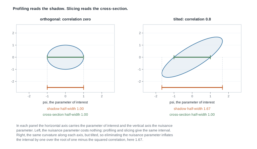
Put numbers on it. Let \(Y_i = \psi z_i + \lambda w_i + \varepsilon_i\) with \(\varepsilon_i\) independent \(N(0, \sigma^2)\) and \(\sigma^2\) known, so the information matrix is proportional to the averaged cross-products of the covariates. Writing \(\rho\) for the sample correlation between \(z\) and \(w\),
\[ i_{\psi\psi \cdot \lambda} = \frac{\overline{z^2}}{\sigma^2}\bigl(1 - \rho^2\bigr), \]
the familiar variance-inflation factor arriving from the likelihood side. At \(\rho = 0.8\) you keep \(1 - 0.64 = 0.36\) of the information an orthogonal design would have given, the standard error of \(\hat\psi\) inflates by \(1/\sqrt{0.36} = 1.67\), and restoring the original precision needs \(1/0.36 = 2.78\) times the sample size. That is not a defect of the profile, which reports a real loss faithfully: a nuisance parameter is expensive exactly when it is hard to tell apart from the parameter you care about.
Conditioning and invariance as other eliminations
The alternatives to profiling are exact where profiling is approximate. The first is conditioning. Suppose that for each fixed \(\psi\) the statistic \(S\) is sufficient for \(\lambda\), as happens in an exponential family where \(\lambda\) is a natural parameter with natural statistic \(S\). Then the conditional distribution of the data given \(S = s\) does not involve \(\lambda\), and the conditional likelihood \(L_{\text{c}}(\psi) = P_{\psi}(X = x \mid S = s)\) is a genuine likelihood for a genuine distribution, free of the nuisance parameter at every sample size rather than in a limit. What conditioning buys is exactness; what it discards is the information about \(\psi\) carried by the marginal distribution of \(S\), and — in discrete problems — a good deal of level, since the conditional distribution offers only finitely many attainable tail probabilities.
The second route is invariance. If a group of transformations carries the model into itself, moving the nuisance parameter while leaving the hypothesis about \(\psi\) unchanged, restrict attention to tests unchanged by them. Such tests depend on the data only through a maximal invariant, whose distribution depends only on the corresponding invariant function of the parameter. For \(X_1, \dots, X_n\) independent \(N(\mu, \sigma^2)\) with both unknown, testing \(H_0 : \mu = 0\) against \(\mu > 0\), the problem is unchanged by \(x \mapsto bx\) for every \(b > 0\); the maximal invariant reduces the data to the \(t\) statistic, whose distribution depends on \((\mu, \sigma)\) only through \(\mu/\sigma\), and that family has a monotone likelihood ratio in \(t\). Week 3’s Karlin-Rubin argument then delivers the \(t\) test as uniformly most powerful among invariant tests — most powerful invariant, not most powerful outright, and the two-sided version needs the reflection \(x \mapsto -x\) in the group as well.
Where profiling stops working
Everything above assumed \(\lambda\) has fixed dimension. Drop that and profiling can fail outright. Let \(X_{ij}\) be independent \(N(\mu_i, \sigma^2)\) for \(i = 1, \dots, n\) and \(j = 1, 2\), with \(\sigma^2\) of interest and one nuisance mean per pair. Profiling out every \(\mu_i\) gives \(\hat\mu_i = \bar{X}_i\) and then
\[ \hat\sigma^2 = \frac{1}{2n}\sum_{i=1}^{n}\sum_{j=1}^{2}\bigl(X_{ij} - \bar{X}_i\bigr)^2 \;\longrightarrow\; \frac{\sigma^2}{2} \]
in probability, because each inner sum has expectation \(\sigma^2\) rather than \(2\sigma^2\): one degree of freedom per pair went into \(\hat\mu_i\) and the profile does not know it. No sample size repairs an estimator that converges to the wrong number. Corrections exist and are worth knowing by name: the modified profile likelihood and the conditional profile likelihood both add an adjustment built from the curvature in \(\lambda\), restoring the missing degrees of freedom, and the Bartlett correction rescales \(\Lambda_P\) so that its mean matches the chi-square mean to higher order. The transfer example below computes one of them where it has a closed form you will recognize at sight.
Local alternatives and asymptotic power
The first half of the week concerned the null; the second concerns what the tests do when it is false. Asymptotic statements are supposed to compare procedures, but against a fixed alternative \(\psi_1 \ne \psi_0\) they refuse to: every consistent test has power tending to one, so two excellent tests and two mediocre ones read alike. Local alternatives repair the comparison by shrinking the alternative toward the null at the rate that keeps the problem hard.
Why a fixed alternative tells you nothing
The rate is forced by the arithmetic of the score. Under \(\psi_n = \psi_0 + h/\sqrt{n}\) the score contribution is of order \(\sqrt{n} \times n^{-1/2} = 1\): the alternative stays a bounded number of standard errors from the null, forever, and power along the sequence tends to a limit strictly between the level and one. That limit is a number worth comparing. Read \(h\) as the drift, the offset of the alternative measured in units of \(n^{-1/2}\), and read its standardized version below — the drift scaled by the square root of the effective information — as how many standard errors of \(\hat\psi\) the alternative sits from the null at the sample size you have. Then the device becomes the familiar power calculation in disguise.
Noncentrality, contiguity, and the three tests
Under the same regularity as before, and along \(\psi_n = \psi_0 + h/\sqrt{n}\) with \(\lambda\) held fixed, each of the profile likelihood-ratio, score, and Wald statistics converges in distribution to
\[ \chi^2_q(\nu), \qquad \nu = h^{\top} i_{\psi\psi \cdot \lambda}(\theta_0)\, h , \]
so the limiting power at level \(\alpha\) is \(P\{\chi^2_q(\nu) > c_{\alpha}\}\) with \(c_\alpha\) the usual central cutoff. Two features matter. First, the noncentrality is built from the effective information, so the power a nuisance parameter costs is precisely the information it costs. Second, all three tests share the limit, which is stronger than it looks: the statistics differ by terms that vanish in probability under the null, and contiguity carries that fact to the alternative. Le Cam’s first lemma supplies it — when the log-likelihood ratio of \(\psi_n\) against \(\psi_0\) converges under the null to a normal law with mean \(-\tau^2/2\) and variance \(\tau^2\), the alternatives are contiguous to the null, and a sequence that is \(o_P(1)\) under one is \(o_P(1)\) under the other.
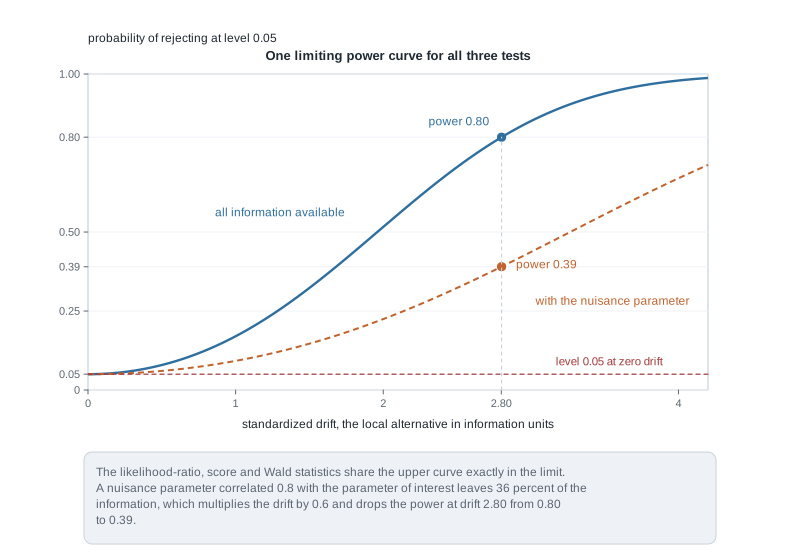
For scalar \(\psi\) at level 0.05 the limiting power is \(P\{\chi^2_1(\nu) > 3.84\}\), which equals \(1 - \Phi(1.96 - \delta) + \Phi(-1.96 - \delta)\) with \(\delta = \sqrt{\nu}\) the standardized drift, the figure’s own horizontal axis, and \(\Phi\) the standard normal distribution function. At \(\delta = 2.80\) that is 0.80, the familiar pairing of eighty percent power with an alternative \(\delta = 2.8\) standard errors from the null. Impose the correlated design of the previous section and \(\delta\) is multiplied by \(\sqrt{1 - \rho^2} = 0.6\), giving \(\delta = 1.68\) and power 0.39: one correlated nuisance parameter has cut the power of the study roughly in half without changing a single observation.
Worked example — profiling the normal mean with unknown variance
The model and the question. A clinical laboratory reports ten independent measurements, modelled as \(X_1, \dots, X_{10}\) independent \(N(\mu, \sigma^2)\) with both parameters unknown:
\[ 4.6,\; 5.2,\; 3.9,\; 4.8,\; 5.5,\; 4.1,\; 5.0,\; 4.4,\; 5.8,\; 4.7 . \]
The interest parameter is \(\psi = \mu\), the nuisance parameter is \(\lambda = \sigma^2\), and the test is \(H_0 : \mu = 4.4\) against the two-sided alternative at level 0.05. The conditions hold: the support does not depend on the parameter, the model is identifiable, the null value is interior, \(\ell\) is smooth, the nuisance parameter is one-dimensional and estimated at rate \(\sqrt{n}\), and the information matrix is positive definite. Here \(\bar{x} = 4.80\), \(\sum (x_i - \bar{x})^2 = 3.20\), \(s^2 = 3.20/9 = 0.3556\), and \(s = 0.5963\).
Step 1, the joint log-likelihood. Dropping constants,
\[ \ell(\mu, \sigma^2) = -\frac{n}{2}\log \sigma^2 - \frac{1}{2\sigma^2}\sum_{i=1}^{n}(x_i - \mu)^2 , \qquad \sum_{i=1}^{n}(x_i - \mu)^2 = \sum_{i=1}^{n}(x_i - \bar{x})^2 + n(\bar{x} - \mu)^2 . \]
Step 2, profile the variance out. For fixed \(\mu\), setting the derivative in \(\sigma^2\) to zero gives \(\hat\sigma^2_\mu = n^{-1}\sum (x_i - \mu)^2\), the ridge in the first figure. Substituting,
\[ \ell_P(\mu) = -\frac{n}{2}\log\Bigl\{\frac{1}{n}\Bigl(\textstyle\sum (x_i - \bar{x})^2 + n(\bar{x} - \mu)^2\Bigr)\Bigr\} - \frac{n}{2}, \]
maximized at \(\hat\mu = \bar{x} = 4.80\), where \(\hat\sigma^2 = 3.20/10 = 0.320\).
Step 3, the profile likelihood-ratio statistic. Taking twice the difference, the constants cancel:
\[ \Lambda_P(\mu_0) = n \log\Bigl(1 + \frac{t^2}{n-1}\Bigr), \qquad t = \frac{\sqrt{n}\,(\bar{x} - \mu_0)}{s} . \]
This is the result the week turns on. \(\Lambda_P\) is a strictly increasing function of \(|t|\), so the profile likelihood-ratio test is the two-sided \(t\) test, ordering the sample space identically: profiling recovered the classical procedure rather than replacing it.
Step 4, the arithmetic. With \(\mu_0 = 4.40\), \(t = \sqrt{10}\,(0.40)/0.5963 = 2.1213\) and \(t^2 = 4.500\) exactly, so \(\Lambda_P = 10\log(1 + 4.5/9) = 10 \log 1.5 = 4.055\).
Step 5, two calibrations of one number. Referred to \(\chi^2_1\) the p-value is 0.044 and the test rejects; referred to the \(t_9\) distribution, exact here, \(|t| = 2.1213\) gives 0.063 and it does not. Only the reference distribution differs, and only one of the two is right at \(n = 10\).
Step 6, the information loss made explicit. Differentiating \(\ell_P\) twice and evaluating at \(\bar{x}\) gives \(-\ell_P''(\bar{x}) = n^2/\sum(x_i - \bar{x})^2 = n/\hat\sigma^2 = 10/0.320 = 31.25\). That is the known-variance information \(n/\sigma^2\) with \(\sigma^2\) replaced by its maximum likelihood estimate — and \(E(\hat\sigma^2) = \sigma^2 (n-1)/n\), so the plug-in is biased low and the curvature biased high. The standard error the profile implies is \(1/\sqrt{31.25} = 0.1789\) against the correct \(s/\sqrt{n} = 0.1886\), too small by the factor \(\sqrt{(n-1)/n} = 0.949\). Here \(\mu\) and \(\sigma^2\) are orthogonal, so the first-order cost is zero and the whole price is paid at order \(1/n\), through this plug-in bias and the reference distribution.
Step 7, the intervals. Inverting the chi-square-calibrated profile test gives 4.413 to 5.187; the exact \(t\) interval is 4.373 to 5.227. The naive interval is about ninety-one percent as wide, and 4.40 falls outside it and inside the exact one. A quadratic fit to the profile, using 1.96 with the curvature above, does worse: 4.449 to 5.151, about eighty-two percent of the correct width.
What this licenses, and what it does not. You may report that these ten measurements are consistent with a mean of 4.40 at the 0.05 level. You may not report the chi-square-calibrated rejection. Notice what rescued the calculation: not the profile, but the exact pivot this model happens to have. Without one you face the same overstatement with no yardstick to measure it against.
x  <- c(4.6, 5.2, 3.9, 4.8, 5.5, 4.1, 5.0, 4.4, 5.8, 4.7)
n  <- length(x)
ss <- sum((x - mean(x))^2)
prof <- function(mu) -0.5 * n * log((ss + n * (mean(x) - mu)^2) / n)   # up to a constant
stat <- 2 * (prof(mean(x)) - prof(4.4))
c(profile_lr = stat,
  chisq_p    = pchisq(stat, df = 1, lower.tail = FALSE),
  exact_t_p  = t.test(x, mu = 4.4)$p.value)
The same reasoning, transferred
Keep the model and the data and swap the roles: let \(\sigma^2\) be the interest parameter and \(\mu\) the nuisance. The recipe is unchanged. For fixed \(\sigma^2\) the best mean is \(\bar{x}\) whatever the variance, so
\[ \ell_P(\sigma^2) = -\frac{n}{2}\log \sigma^2 - \frac{\sum (x_i - \bar{x})^2}{2\sigma^2}, \]
maximized at \(\hat\sigma^2 = \sum (x_i - \bar{x})^2/n = 0.320\). What stayed the same: one parameter removed by maximization, one curve left over, a nuisance parameter estimated rather than known. What changed is where the damage shows. In the first direction the point estimate was fine and the reference distribution wrong; here the point estimate itself is biased, since \(E(\hat\sigma^2) = 0.9\,\sigma^2\) at \(n = 10\).
This is the case where the adjustment has a closed form. The conditional profile likelihood adds \(-\tfrac{1}{2}\log |J_{\lambda\lambda}(\sigma^2, \hat\mu)|\) to \(\ell_P\), and here \(J_{\mu\mu} = n/\sigma^2\), so the adjustment contributes \(\tfrac{1}{2}\log \sigma^2\) up to a constant:
\[ \ell_{\text{adj}}(\sigma^2) = -\frac{n-1}{2}\log\sigma^2 - \frac{\sum (x_i - \bar{x})^2}{2\sigma^2}, \]
whose maximizer is \(\sum (x_i - \bar{x})^2/(n-1) = s^2 = 0.3556\), the unbiased estimator. The correction did nothing more mysterious than notice that estimating the mean spent one observation’s worth of information, and the denominator \(n - 1\) is the receipt.
Second worked example — conditioning away the nuisance in a two-by-two table
The model and the question. A field trial applies a treatment to seven units and a control to seven others, with five successes in the treated group and one in the control group. Model the counts as independent \(X \sim \text{Binomial}(7, p_A)\) and \(Y \sim \text{Binomial}(7, p_B)\), and write the parameters as the log odds ratio \(\psi = \log\{p_A(1 - p_B)/((1 - p_A)p_B)\}\), of interest, and \(\lambda = \log\{p_B/(1 - p_B)\}\), the baseline log odds, a nuisance. The null of no treatment effect is \(H_0 : \psi = 0\), with \(\lambda\) unknown under both hypotheses.
Step 1, find the sufficient statistic for the nuisance. In exponential-family form,
\[ P(X = x, Y = y) = \binom{7}{x}\binom{7}{y} \frac{\exp\{\psi x + \lambda (x + y)\}} {(1 + e^{\psi + \lambda})^{7}\,(1 + e^{\lambda})^{7}} , \]
so for each fixed \(\psi\) the total \(S = X + Y\) is sufficient for \(\lambda\). That is the structural fact conditioning needs, and it is exact rather than asymptotic.
Step 2, condition. Dividing by the marginal probability of \(S = s\) cancels every factor carrying \(\lambda\) and leaves
\[ P(X = k \mid S = s) = \frac{\binom{7}{k}\binom{7}{s-k} e^{\psi k}} {\sum_{j}\binom{7}{j}\binom{7}{s-j} e^{\psi j}} , \]
which involves \(\psi\) alone. At \(\psi = 0\) this is the hypergeometric distribution over tables with the observed margins, and the test built from it is Fisher’s exact test.
Step 3, the exact tail by counting. Here \(s = 6\) and both groups have seven units, so the denominator is \(\binom{14}{6} = 3003\) and the numerators \(\binom{7}{k}\binom{7}{6-k}\) for \(k = 0, \dots, 6\) are 7, 147, 735, 1225, 735, 147, 7. The observed \(k = 5\) has probability \(147/3003\), and
\[ P(X \ge 5 \mid S = 6) = \frac{147 + 7}{3003} = \frac{154}{3003} = \frac{2}{39} = 0.0513 . \]
The null distribution is symmetric because the group sizes are equal, so the two-sided exact p-value is \(4/39 = 0.1026\); collecting the outcomes at least as improbable as the observed one selects the same four tables and the same number.
Step 4, compare with the approximations. Each large-sample statistic below eliminates the nuisance parameter by maximizing rather than conditioning.
| Procedure | Statistic | p-value |
|---|---|---|
| Exact conditional, two-sided | tail probability by counting | 0.1026 |
| Wald on the log odds ratio | \(3.929\) | 0.0475 |
| Pearson chi-square | \(4.667\) | 0.0308 |
| Likelihood ratio, profiled | \(5.004\) | 0.0253 |
The Wald entry uses \(\hat\psi = \log\{(5)(6)/((2)(1))\} = \log 15 = 2.708\) with standard error \(\sqrt{1/5 + 1/2 + 1/1 + 1/6} = 1.366\), giving \((2.708/1.366)^2 = 3.929\); the Pearson statistic uses expected counts 3, 4, 3, 4 under independence; the profiled likelihood-ratio statistic is \(2\sum O \log(O/E)\) over the same four cells. Every approximation lands below 0.05, the exact calculation well above it, and the approximations disagree among themselves by nearly a factor of two.
Step 5, what the reduction discards. Conditioning is not free. The margin \(S\) is not entirely uninformative about \(\psi\), so its distribution carries information the conditional analysis throws away, and correspondingly the conditional maximum likelihood estimate of the log odds ratio, 2.461 by numerical solving, is shrunk relative to the unconditional 2.708. Discreteness costs more: with these margins the attainable two-sided conditional p-values are 0.0047 and 0.1026 and nothing between, so a level-0.05 exact test here has conditional size 0.0047, valid but conservative by a factor of ten. That is the conservatism Week 4 met when inverting exact binomial tests.
tab <- matrix(c(5, 2, 1, 6), nrow = 2, byrow = TRUE)   # rows: treated, control
fisher.test(tab)$p.value                               # exact conditional, two-sided
chisq.test(tab, correct = FALSE)$p.value               # Pearson, chi-square reference
dhyper(0:6, 7, 7, 6)                                   # the whole conditional null
What this licenses, and what it does not. You may report that these fourteen units supply no evidence against the null at the 0.05 level once the baseline rate is eliminated exactly. You may not report the chi-square p-value as though it described the same evidence, nor treat the conservatism as a feature: a test with actual size 0.0047 buys exactness with power a larger trial need not have spent.
The misreading to avoid
The sentence to dismantle is this one: “I profiled out the nuisance parameters, so the profile is my likelihood now — I can read intervals off its curvature and refer twice its drop to a chi-square, the same as always.” The first clause describes a calculation correctly; everything after it imports a guarantee that was never transferred.
A profile likelihood is a maximized value, not a probability model. No density has it as its log-likelihood, so the identities that make likelihood inference work — a score with mean zero, a variance matching the information — hold only to first order. The curvature identity above is reassuring at that order, since it shows the profile already discounting the uncertainty in \(\hat\lambda\). But at \(n = 10\) the discount plugs in an estimate biased low, and the resulting interval covered 0.930 rather than 0.950 above, with the cruder quadratic version covering 0.904.
The second misreading comes from the local-alternative theory: “the three tests have the same limiting power, so choosing among them is a matter of taste.” The limiting power function is shared; the finite-sample behaviour is not, and last week’s example put 3.139, 3.000, and 4.000 on the same twelve observations. The shared limit is also built from the effective information, so the theorem is silent about the comparison that matters most here, profiling against conditioning, which turns on exactness at your sample size rather than on a common limit.
The third misreads the local sequence itself. Local alternatives are not a claim that effects shrink as data accumulate, and power computed along the sequence is not a probability about your study: it approximates the power at an alternative \(\delta\) standard errors from the null, for the drift \(h\) and the sample size you have, and is only as good as the normal approximation underneath. When someone calls a test asymptotically efficient, ask which sequence of alternatives, which information, and at what sample size the promise begins to bind.
Practice on your own
These are for self-checking; work them before the calibration lab rather than after.
- The curvature identity, by hand. For the two-parameter normal model above, compute all four entries of \(J\) at the maximum and verify that \(J_{\mu\mu} - J_{\mu\sigma^2}J_{\sigma^2\sigma^2}^{-1}J_{\sigma^2\mu}\) equals the 31.25 obtained by differentiating \(\ell_P\) directly. Say why the cross term vanished.
- A non-orthogonal profile. In the two-covariate linear model take \(n = 40\), \(\overline{z^2} = 1\), \(\sigma^2 = 1\), and \(\rho\) equal to 0, then 0.5, then 0.9. Report the effective information, the standard error of \(\hat\psi\), the limiting power at drift \(h = 2.8\), and the sample size needed at \(\rho = 0.9\) to match the power at \(\rho = 0\).
- Exact against approximate. Construct a two-by-two table whose Fisher and Pearson p-values fall on opposite sides of 0.05, then one where the ordering reverses. Enumerate the conditional null in both cases and say which feature of the margins drives the disagreement.
- A profile that misleads badly. Simulate the matched design of the last concept section with \(n = 50\) pairs and \(\sigma^2 = 1\), and confirm the profile estimate concentrates near one half. Apply the degrees-of-freedom correction, then repeat with four observations per pair and explain why the bias shrinks.
- Coverage of a profile interval. Reproduce the coverage figure at \(n = 8\) and \(n = 25\) below and report the Monte Carlo standard error of each estimate. Predict, before running it, what changes if the cutoff 3.84 is replaced by the exactly calibrated one.
set.seed(2027)
covered <- function(n, reps = 20000) {
  mean(replicate(reps, {
    z  <- rnorm(n)
    ss <- sum((z - mean(z))^2)
    n * log(1 + n * mean(z)^2 / ss) <= qchisq(0.95, df = 1)
  }))
}
c(n8 = covered(8), n25 = covered(25))
Where to read more
- The large-sample likelihood theory this week extends, including nuisance parameters and the local-alternative calculations, is developed in the lecture materials for MIT OpenCourseWare 18.655 Mathematical Statistics.
- A slower, example-first treatment of the \(t\) procedures and of exact tests for tables, useful if the profile derivation moved quickly, is in Penn State STAT 415.
- The optional Hogg, McKean, and Craig alignment for this week is Chapter 5 together with Chapter 6.4 and 6.5. That book is optional and is never required to be purchased.
- Everything computed here uses base R and the
statspackage only; see The R Project for Statistical Computing and Quarto. - Course pages: the syllabus, the schedule, the resources overview, and the notes overview. The three statistics profiled here were built in Week 5, and the conservatism of the exact conditional test is the phenomenon met in Week 4.
Where this goes next
Week 7 consolidates the first half of the course into a procedure you can follow when a problem arrives without a label on it: what to ask first, how to choose between an exact and an approximate route, and how to run a size-and-power study that says whether your approximation is calibrated at the sample size you have. This week supplies two of the questions on that list. Which parameters are nuisance, and how are they being eliminated? And is the reference distribution I am about to use the one that belongs to the statistic I actually computed?
Two threads continue past the midpoint. Week 8 returns to the normal linear model and shows that the degrees of freedom lost to a nuisance parameter here are ranks of projections there. Week 10 turns the conditioning argument of the second worked example into a general principle, deriving validity from the design rather than from a distributional assumption. If a step went past you, rebuild the curvature identity first, since the rest of the profile story follows from it; the notes overview lists the earlier units.